🎬 OPENING SCENE

png

The Challenge: Security vs. Sanity

The Numbers Don’t Lie (But Fraudsters Do)

60% of financial organizations reported an increase in fraud.
1 in 4 people have experienced payment fraud
24/7 - Fraudsters are always online (they don’t have a 9-5 job)
FALSE POSITIVES - Legit customers getting blocked feels WORSE than getting hacked.

Think about it: You’re at the grocery store. You try to pay. DECLINED . You just got Sarah’d. And now you’re embarrassed. And angry. And hungry.

What are we doing in this notebook?

We are stepping into the shoes of a fraud analytics team at a digital payments company.
Our mission: Spot suspicious transactions fast enough that people like Sarah never lose a dollar.

Think of this notebook as a mix of:

a crime investigation story
a data science lab
and a model-building workshop

Along the way, we will:

get to know our cast of characters (features, devices, email domains, cards)
interrogate suspicious behavior through EDA
and train models to separate legit from fraud with as little confusion as possible.

Project Roadmap

PHASE 1: THE EVIDENCE (Data Collection)

1.1 Importing the Toolkit
1.2 Loading the Raw Logs

PHASE 2: SANITIZING THE DATA (Preprocessing)

2.1 Consistency Check (Duplicates)
2.2 Parsing Data Types
2.3 Handling Missing Intelligence

PHASE 3: THE INVESTIGATION (Exploratory Analysis)

3.1: Descriptive Statistics & Frequency Analysis
3.2: Correlation Analysis
3.3: Hypothesis Testing & Outlier Analysis
3.4: Temporal Analysis (Time Patterns)

PHASE 4: THE DETECTIVES (Machine Learning)

4.1 Feature Encoding & Data Split
4.2 Building the Basic Detector: Logistic Regression
4.3 Random Forest Classifier
4.4 XGBoost
4.5 Evaluating our fraud detector: Beyond plain accuracy

PHASE 5: EVALUATING ON UNSEEN DATA

FUTURE WORK

REFERENCES & RECOURCES

DATA COLLECTION

The Data

Every investigation begins with data collection. And for our detective work we need real live payment systems data harvested under strict privacy constraints. Hence we have chosen IEEE-CIS Fraud Detection data from Kaggle.

Who created this data?

Vesta Corporation - A fraud prevention company
IEEE Computational Intelligence Society - For education & research
Anonymized real payment transaction data

Why this dataset?

Real-world scale: 500,000+ transactions (not a toy dataset)
Complex features: 240+ columns capturing every angle of fraud
Business relevance: Used by actual fraud detection teams
Balanced scope: Big enough to learn from, small enough to run locally

If you are unfamiliar with Kaggle, it is like “GitHub for data scientists” - a platform where companies post real datasets and challenges. Data scientists compete to build the best models. It’s how professionals practice, learn, and showcase skills.

Think of it as:

Real-world data (not fake textbook examples)
Data cleaned by professionals (Vesta Corporation in this case)
Problems that actually matter (fraud costs billions annually)

The Data Architecture

To catch a thief, we need to look at the full picture. Our dataset is a relationship between two distinct stories linked by a TransactionID.

1. The Paper Trail (Transaction Table)

This is the “what” and the “where.” It holds the details you’d expect on a receipt:

The Basics: Product codes and card information (card1 - card6).
The User: Email domains (gmail.com, etc.) and billing locations.
The Clock: A time-delta (TransactionDT) that tells us when it happened relative to a start date.

2. The Digital Fingerprint (Identity Table)

This is the “who” (or “what machine”). It captures the hidden network details:

The Device: Is it a phone? A desktop? What specific model? (DeviceType, DeviceInfo).
The Network: Anonymized technical attributes that act like digital breadcrumbs.

The Split

We teach the model using a Training Set (where we already know who the fraudsters are) and then grade its performance on a Test Set (unseen data) to ensure it can handle the real world.

1.1 Importing the Toolkit

First, we need to gather our tools. We’re importing the standard data science stack to help us wrangle the raw data and visualize the hidden patterns inside.

Meet our toolbox

Before we interrogate any suspicious transaction, we need our investigation gear:

pandas → our data detective reading CSV files and cleaning up the mess
numpy → the math engine handling numbers behind the scenes
matplotlib / seaborn → the visual storytellers turning patterns into plots
sklearn → the model workshop, where we test algorithms and tune them like race cars

Once the toolkit is ready, we can invite the data into the lab.

New to these libraries? Explore the official documentation for pandas, numpy, matplotlib, seaborn, and scikit-learn to dive deeper into each powerful tool.

import os
import gc
import math
import numpy as np
import pandas as pd
from google.colab import drive

# plotting
import matplotlib.pyplot as plt
import seaborn as sns

# stats/tests
from scipy import stats
from sklearn.experimental import enable_iterative_imputer
from sklearn.impute import SimpleImputer, IterativeImputer
from sklearn.preprocessing import LabelEncoder, StandardScaler
from sklearn.model_selection import train_test_split
from sklearn.linear_model import LogisticRegression
from sklearn.pipeline import make_pipeline
from sklearn.metrics import accuracy_score, roc_auc_score, classification_report, confusion_matrix, roc_curve , precision_recall_curve , auc , f1_score , precision_score , recall_score
from sklearn.ensemble import RandomForestClassifier
from sklearn.tree import plot_tree
import xgboost as xgb

# settings
pd.set_option('display.max_rows', 100)
pd.set_option('display.max_columns', 500)
sns.set(style="whitegrid")
plt.rcParams["figure.figsize"] = (10, 5)
RANDOM_STATE = 42

drive.mount('/content/drive')

Mounted at /content/drive

1.2 Loading the Raw Logs

Time to bring in the evidence. We load the raw transaction and identity logs to begin looking for clues.

# load files
tx_train_path = "/content/drive/MyDrive/602-Project/train_transaction.csv"
id_train_path = "/content/drive/MyDrive/602-Project/train_identity.csv"

print("Files exist:", os.path.exists(tx_train_path), os.path.exists(id_train_path))

Files exist: True True

1.2.1 Transaction & Identity Data

df_tx_train = pd.read_csv(tx_train_path, low_memory=False)

df_tx_train.head(10)

	TransactionID	TransactionDT	TransactionAmt	ProductCD	card1	card2	card3	card4	card5	card6	addr1	addr2	dist1	dist2	P_emaildomain	R_emaildomain	C1	C2	C6	C8	C9	C10	C11	C13	C14	D1	D2	D3	D4	D5	D6	D7	D8	D9	D10	D11	D12	D13	D14	D15	M1	M2	M3	M4	M5	M6	M7	M8	M9	V1	V2	V3	V4	V5	V6	V7	V8	V9	V10	V11	V12	V13	V14	V15	V16	V17	V18	V19	V20	V21	V22	V23	V24	V25	V26	V27	V28	V29	V30	V31	V32	V33	V34	V35	V36	V37	V38	V39	V40	V41	V42	V43	V44	V45	V46	V47	V48	V49	V50	V51	V52	V53	V54	V55	V56	V57	V58	V59	V60	V61	V62	V63	V64	V65	V66	V67	V68	V69	V70	V71	V72	V73	V74	V75	V76	V77	V78	V79	V80	V81	V82	V83	V84	V85	V86	V87	V88	V89	V90	V91	V92	V93	V94	V95	V96	V97	V99	V100	V101	V102	V103	V107	V108	V109	V110	V111	V112	V113	V114	V115	V116	V117	V118	V119	V120	V121	V122	V123	V124	V125	V126	V127	V128	V130	V131	V132	V133	V134	V138	V139	V140	V141	V142	V143	V144	V145	V146	V147	V148	V149	V150	V151	V152	V153	V154	V155	V156	V157	V158	V159	V160	V161	V162	V163	V164	V165	V166	V167	V168	V169	V170	V171	V172	V173	V174	V175	V176	V177	V178	V179	V180	V181	V182	V183	V184	V185	V186	V187	V188	V189	V190	V191	V192	V193	V194	V195	V196	V197	V198	V199	V200	V201	V202	V203	V204	V205	V206	V207	V208	V209	V210	V211	V212	V213	V214	V215	V216	V217	V218	V219	V220	V221	V222	V223	V224	V225	V226	V227	V228	V229	V230	V231	V232	V233	V234	V235	V236	V237	V238	V239	V240	V241	V242	V243	V244	V245	V246	V247	V248	V249	V250	V251	V252	V253	V254	V255	V256	V257	V258	V259	V260	V261	V262	V263	V264	V265	V266	V267	V268	V269	V270	V271	V272	V273	V274	V275	V276	V277	V278	V279	V280	V282	V283	V285	V287	V290	V291	V292	V293	V294	V295	V302	V303	V304	V305	V306	V307	V308	V310	V312	V314	V316	V317	V318	V322	V323	V324	V325	V326	V327	V328	V329	V330	V331	V332	V333	V334	V335	V336	V337	V338	V339
0	2987000	86400	68.5	W	13926	NaN	150.0	discover	142.0	credit	315.0	87.0	19.0	NaN	NaN	NaN	1.0	1.0	1.0	0.0	1.0	0.0	2.0	1.0	1.0	14.0	NaN	13.0	NaN	NaN	NaN	NaN	NaN	NaN	13.0	13.0	NaN	NaN	NaN	0.0	T	T	T	M2	F	T	NaN	NaN	NaN	1.0	1.0	1.0	1.0	1.0	1.0	1.0	1.0	1.0	0.0	0.0	1.0	1.0	1.0	0.0	0.0	0.0	0.0	1.0	1.0	0.0	0.0	1.0	1.0	1.0	1.0	0.0	0.0	0.0	0.0	0.0	0.0	0.0	0.0	NaN	NaN	NaN	NaN	NaN	NaN	NaN	NaN	NaN	NaN	NaN	NaN	NaN	NaN	NaN	NaN	NaN	NaN	1.0	1.0	1.0	1.0	0.0	0.0	0.0	0.0	1.0	1.0	0.0	0.0	1.0	1.0	1.0	0.0	0.0	0.0	0.0	0.0	0.0	0.0	1.0	1.0	1.0	1.0	0.0	0.0	0.0	0.0	0.0	0.0	0.0	1.0	1.0	1.0	0.0	0.0	0.0	0.0	0.0	0.0	0.0	1.0	0.0	0.0	0.0	0.0	1.0	0.0	1.0	1.0	1.0	1.0	1.0	1.0	1.0	1.0	1.0	1.0	1.0	1.0	1.0	1.0	1.0	1.0	1.0	1.0	1.0	0.0	117.0	0.0	0.0	0.0	0.0	117.0	0.0	NaN	NaN	NaN	NaN	NaN	NaN	NaN	NaN	NaN	NaN	NaN	NaN	NaN	NaN	NaN	NaN	NaN	NaN	NaN	NaN	NaN	NaN	NaN	NaN	NaN	NaN	NaN	NaN	NaN	NaN	NaN	NaN	NaN	NaN	NaN	NaN	NaN	NaN	NaN	NaN	NaN	NaN	NaN	NaN	NaN	NaN	NaN	NaN	NaN	NaN	NaN	NaN	NaN	NaN	NaN	NaN	NaN	NaN	NaN	NaN	NaN	NaN	NaN	NaN	NaN	NaN	NaN	NaN	NaN	NaN	NaN	NaN	NaN	NaN	NaN	NaN	NaN	NaN	NaN	NaN	NaN	NaN	NaN	NaN	NaN	NaN	NaN	NaN	NaN	NaN	NaN	NaN	NaN	NaN	NaN	NaN	NaN	NaN	NaN	NaN	NaN	NaN	NaN	NaN	NaN	NaN	NaN	NaN	NaN	NaN	NaN	NaN	NaN	NaN	NaN	NaN	NaN	NaN	NaN	NaN	NaN	NaN	NaN	NaN	NaN	NaN	NaN	NaN	NaN	NaN	NaN	NaN	NaN	NaN	NaN	NaN	NaN	NaN	NaN	NaN	NaN	0.0	0.0	1.0	1.0	0.0	0.0	1.0	1.0	1.0	0.0	1.0	0.0	0.0	0.0	0.0	1.0	0.0	117.0	0.0	0.0	0.0	0.0	0.0	117.0	0.0	NaN	NaN	NaN	NaN	NaN	NaN	NaN	NaN	NaN	NaN	NaN	NaN	NaN	NaN	NaN	NaN	NaN	NaN
1	2987001	86401	29.0	W	2755	404.0	150.0	mastercard	102.0	credit	325.0	87.0	NaN	NaN	gmail.com	NaN	1.0	1.0	1.0	0.0	0.0	0.0	1.0	1.0	1.0	0.0	NaN	NaN	0.0	NaN	NaN	NaN	NaN	NaN	0.0	NaN	NaN	NaN	NaN	0.0	NaN	NaN	NaN	M0	T	T	NaN	NaN	NaN	NaN	NaN	NaN	NaN	NaN	NaN	NaN	NaN	NaN	NaN	NaN	0.0	0.0	1.0	0.0	0.0	0.0	0.0	1.0	1.0	0.0	0.0	1.0	1.0	1.0	1.0	0.0	0.0	0.0	0.0	0.0	0.0	0.0	0.0	0.0	0.0	1.0	1.0	0.0	0.0	1.0	0.0	0.0	1.0	1.0	1.0	1.0	0.0	0.0	0.0	0.0	0.0	0.0	0.0	1.0	1.0	0.0	0.0	0.0	0.0	1.0	1.0	0.0	0.0	1.0	1.0	1.0	0.0	0.0	0.0	0.0	0.0	0.0	0.0	0.0	0.0	1.0	1.0	0.0	0.0	0.0	1.0	1.0	0.0	0.0	1.0	1.0	1.0	0.0	0.0	0.0	0.0	0.0	0.0	0.0	0.0	0.0	0.0	0.0	0.0	0.0	0.0	1.0	1.0	1.0	1.0	1.0	1.0	1.0	1.0	1.0	1.0	1.0	1.0	1.0	1.0	1.0	1.0	1.0	1.0	1.0	0.0	0.0	0.0	0.0	0.0	0.0	0.0	0.0	NaN	NaN	NaN	NaN	NaN	NaN	NaN	NaN	NaN	NaN	NaN	NaN	NaN	NaN	NaN	NaN	NaN	NaN	NaN	NaN	NaN	NaN	NaN	NaN	NaN	NaN	NaN	NaN	NaN	NaN	NaN	NaN	NaN	NaN	NaN	NaN	NaN	NaN	NaN	NaN	NaN	NaN	NaN	NaN	NaN	NaN	NaN	NaN	NaN	NaN	NaN	NaN	NaN	NaN	NaN	NaN	NaN	NaN	NaN	NaN	NaN	NaN	NaN	NaN	NaN	NaN	NaN	NaN	NaN	NaN	NaN	NaN	NaN	NaN	NaN	NaN	NaN	NaN	NaN	NaN	NaN	NaN	NaN	NaN	NaN	NaN	NaN	NaN	NaN	NaN	NaN	NaN	NaN	NaN	NaN	NaN	NaN	NaN	NaN	NaN	NaN	NaN	NaN	NaN	NaN	NaN	NaN	NaN	NaN	NaN	NaN	NaN	NaN	NaN	NaN	NaN	NaN	NaN	NaN	NaN	NaN	NaN	NaN	NaN	NaN	NaN	NaN	NaN	NaN	NaN	NaN	NaN	NaN	NaN	NaN	NaN	NaN	NaN	NaN	NaN	NaN	0.0	0.0	1.0	1.0	0.0	0.0	1.0	1.0	1.0	0.0	0.0	0.0	0.0	0.0	0.0	1.0	0.0	0.0	0.0	0.0	0.0	0.0	0.0	0.0	0.0	NaN	NaN	NaN	NaN	NaN	NaN	NaN	NaN	NaN	NaN	NaN	NaN	NaN	NaN	NaN	NaN	NaN	NaN
2	2987002	86469	59.0	W	4663	490.0	150.0	visa	166.0	debit	330.0	87.0	287.0	NaN	outlook.com	NaN	1.0	1.0	1.0	0.0	1.0	0.0	1.0	1.0	1.0	0.0	NaN	NaN	0.0	NaN	NaN	NaN	NaN	NaN	0.0	315.0	NaN	NaN	NaN	315.0	T	T	T	M0	F	F	F	F	F	1.0	1.0	1.0	1.0	1.0	1.0	1.0	1.0	1.0	0.0	0.0	1.0	1.0	1.0	0.0	0.0	0.0	0.0	1.0	1.0	0.0	0.0	1.0	1.0	1.0	1.0	0.0	0.0	0.0	0.0	0.0	0.0	0.0	0.0	1.0	1.0	1.0	1.0	0.0	0.0	1.0	0.0	0.0	1.0	1.0	1.0	1.0	0.0	0.0	0.0	0.0	0.0	1.0	1.0	1.0	1.0	0.0	0.0	0.0	0.0	1.0	1.0	0.0	0.0	1.0	1.0	1.0	0.0	0.0	0.0	0.0	0.0	0.0	0.0	1.0	1.0	1.0	1.0	0.0	0.0	0.0	1.0	1.0	0.0	0.0	1.0	1.0	1.0	0.0	0.0	0.0	0.0	0.0	0.0	0.0	0.0	0.0	0.0	0.0	0.0	0.0	0.0	1.0	1.0	1.0	1.0	1.0	1.0	1.0	1.0	1.0	1.0	1.0	1.0	1.0	1.0	1.0	1.0	1.0	1.0	1.0	0.0	0.0	0.0	0.0	0.0	0.0	0.0	0.0	NaN	NaN	NaN	NaN	NaN	NaN	NaN	NaN	NaN	NaN	NaN	NaN	NaN	NaN	NaN	NaN	NaN	NaN	NaN	NaN	NaN	NaN	NaN	NaN	NaN	NaN	NaN	NaN	NaN	NaN	NaN	NaN	NaN	NaN	NaN	NaN	NaN	NaN	NaN	NaN	NaN	NaN	NaN	NaN	NaN	NaN	NaN	NaN	NaN	NaN	NaN	NaN	NaN	NaN	NaN	NaN	NaN	NaN	NaN	NaN	NaN	NaN	NaN	NaN	NaN	NaN	NaN	NaN	NaN	NaN	NaN	NaN	NaN	NaN	NaN	NaN	NaN	NaN	NaN	NaN	NaN	NaN	NaN	NaN	NaN	NaN	NaN	NaN	NaN	NaN	NaN	NaN	NaN	NaN	NaN	NaN	NaN	NaN	NaN	NaN	NaN	NaN	NaN	NaN	NaN	NaN	NaN	NaN	NaN	NaN	NaN	NaN	NaN	NaN	NaN	NaN	NaN	NaN	NaN	NaN	NaN	NaN	NaN	NaN	NaN	NaN	NaN	NaN	NaN	NaN	NaN	NaN	NaN	NaN	NaN	NaN	NaN	NaN	NaN	NaN	NaN	0.0	0.0	1.0	1.0	0.0	0.0	1.0	1.0	1.0	0.0	0.0	0.0	0.0	0.0	0.0	1.0	0.0	0.0	0.0	0.0	0.0	0.0	0.0	0.0	0.0	NaN	NaN	NaN	NaN	NaN	NaN	NaN	NaN	NaN	NaN	NaN	NaN	NaN	NaN	NaN	NaN	NaN	NaN
3	2987003	86499	50.0	W	18132	567.0	150.0	mastercard	117.0	debit	476.0	87.0	NaN	NaN	yahoo.com	NaN	2.0	5.0	4.0	0.0	1.0	0.0	1.0	25.0	1.0	112.0	112.0	0.0	94.0	0.0	NaN	NaN	NaN	NaN	84.0	NaN	NaN	NaN	NaN	111.0	NaN	NaN	NaN	M0	T	F	NaN	NaN	NaN	NaN	NaN	NaN	NaN	NaN	NaN	NaN	NaN	NaN	NaN	NaN	1.0	1.0	1.0	0.0	0.0	0.0	0.0	1.0	1.0	0.0	0.0	1.0	1.0	1.0	1.0	0.0	0.0	0.0	0.0	0.0	0.0	0.0	0.0	1.0	1.0	1.0	1.0	0.0	0.0	1.0	0.0	0.0	1.0	1.0	1.0	1.0	0.0	0.0	0.0	0.0	0.0	1.0	1.0	1.0	1.0	0.0	0.0	0.0	0.0	1.0	1.0	0.0	0.0	1.0	1.0	1.0	0.0	0.0	0.0	0.0	0.0	0.0	0.0	1.0	1.0	1.0	1.0	0.0	0.0	0.0	1.0	1.0	0.0	0.0	1.0	1.0	1.0	0.0	0.0	0.0	0.0	0.0	0.0	1.0	48.0	28.0	10.0	4.0	1.0	38.0	24.0	1.0	1.0	1.0	1.0	1.0	1.0	1.0	1.0	1.0	1.0	1.0	1.0	1.0	1.0	1.0	1.0	1.0	1.0	1.0	50.0	1758.0	925.0	354.0	135.0	50.0	1404.0	790.0	NaN	NaN	NaN	NaN	NaN	NaN	NaN	NaN	NaN	NaN	NaN	NaN	NaN	NaN	NaN	NaN	NaN	NaN	NaN	NaN	NaN	NaN	NaN	NaN	NaN	NaN	NaN	NaN	NaN	NaN	NaN	NaN	NaN	NaN	NaN	NaN	NaN	NaN	NaN	NaN	NaN	NaN	NaN	NaN	NaN	NaN	NaN	NaN	NaN	NaN	NaN	NaN	NaN	NaN	NaN	NaN	NaN	NaN	NaN	NaN	NaN	NaN	NaN	NaN	NaN	NaN	NaN	NaN	NaN	NaN	NaN	NaN	NaN	NaN	NaN	NaN	NaN	NaN	NaN	NaN	NaN	NaN	NaN	NaN	NaN	NaN	NaN	NaN	NaN	NaN	NaN	NaN	NaN	NaN	NaN	NaN	NaN	NaN	NaN	NaN	NaN	NaN	NaN	NaN	NaN	NaN	NaN	NaN	NaN	NaN	NaN	NaN	NaN	NaN	NaN	NaN	NaN	NaN	NaN	NaN	NaN	NaN	NaN	NaN	NaN	NaN	NaN	NaN	NaN	NaN	NaN	NaN	NaN	NaN	NaN	NaN	NaN	NaN	NaN	NaN	NaN	1.0	28.0	0.0	0.0	10.0	4.0	1.0	1.0	1.0	1.0	38.0	24.0	0.0	0.0	0.0	1.0	50.0	1758.0	925.0	354.0	135.0	0.0	50.0	1404.0	790.0	NaN	NaN	NaN	NaN	NaN	NaN	NaN	NaN	NaN	NaN	NaN	NaN	NaN	NaN	NaN	NaN	NaN	NaN
4	2987004	86506	50.0	H	4497	514.0	150.0	mastercard	102.0	credit	420.0	87.0	NaN	NaN	gmail.com	NaN	1.0	1.0	1.0	1.0	0.0	1.0	1.0	1.0	1.0	0.0	NaN	NaN	NaN	NaN	NaN	NaN	NaN	NaN	NaN	NaN	NaN	NaN	NaN	NaN	NaN	NaN	NaN	NaN	NaN	NaN	NaN	NaN	NaN	NaN	NaN	NaN	NaN	NaN	NaN	NaN	NaN	NaN	NaN	NaN	NaN	NaN	NaN	NaN	NaN	NaN	NaN	NaN	NaN	NaN	NaN	NaN	NaN	NaN	NaN	NaN	NaN	NaN	NaN	NaN	NaN	NaN	NaN	NaN	NaN	NaN	NaN	NaN	NaN	NaN	NaN	NaN	NaN	NaN	NaN	NaN	NaN	NaN	NaN	NaN	NaN	NaN	NaN	NaN	NaN	NaN	NaN	NaN	NaN	NaN	NaN	NaN	NaN	NaN	NaN	NaN	NaN	NaN	NaN	NaN	NaN	NaN	NaN	NaN	NaN	NaN	NaN	NaN	NaN	NaN	NaN	NaN	NaN	NaN	NaN	NaN	NaN	NaN	NaN	NaN	NaN	NaN	NaN	0.0	0.0	0.0	0.0	0.0	0.0	0.0	0.0	1.0	1.0	1.0	1.0	1.0	1.0	1.0	1.0	1.0	1.0	1.0	1.0	1.0	1.0	1.0	1.0	1.0	1.0	1.0	0.0	0.0	0.0	0.0	0.0	0.0	0.0	0.0	0.0	0.0	0.0	0.0	0.0	6.0	18.0	140.0	0.0	0.0	0.0	0.0	1803.0	49.0	64.0	0.0	0.0	0.0	0.0	0.0	0.0	15557.990234	169690.796875	0.0	0.0	0.0	515.0	5155.0	2840.0	0.0	0.0	0.0	1.0	1.0	0.0	0.0	0.0	0.0	1.0	0.0	0.0	0.0	0.0	0.0	0.0	0.0	0.0	0.0	1.0	1.0	1.0	1.0	1.0	1.0	1.0	1.0	1.0	1.0	1.0	1.0	1.0	1.0	1.0	1.0	0.0	0.0	0.0	0.0	0.0	0.0	0.0	0.0	0.0	0.0	0.0	0.0	0.0	0.0	0.0	0.0	0.0	0.0	0.0	1.0	1.0	0.0	0.0	0.0	0.0	0.0	1.0	1.0	1.0	0.0	0.0	0.0	0.0	0.0	0.0	0.0	0.0	0.0	1.0	1.0	1.0	1.0	1.0	1.0	1.0	1.0	1.0	1.0	1.0	1.0	1.0	1.0	1.0	1.0	1.0	1.0	1.0	1.0	1.0	1.0	1.0	0.0	0.0	0.0	0.0	0.0	0.0	0.0	0.0	0.0	0.0	0.0	0.0	0.0	0.0	0.0	0.0	0.0	0.0	1.0	1.0	0.0	0.0	1.0	1.0	1.0	0.0	0.0	0.0	1.0	1.0	1.0	1.0	0.0	0.0	0.0	0.0	0.0	0.0	0.0	0.0	0.0	0.0	0.0	0.0	0.0	0.0	0.0	0.0	0.0	0.0	0.0	0.0	0.0	0.0	0.0	0.0	0.0	0.0	0.0
5	2987005	86510	49.0	W	5937	555.0	150.0	visa	226.0	debit	272.0	87.0	36.0	NaN	gmail.com	NaN	1.0	1.0	1.0	0.0	1.0	0.0	1.0	1.0	1.0	0.0	NaN	NaN	0.0	NaN	NaN	NaN	NaN	NaN	0.0	0.0	NaN	NaN	NaN	0.0	T	T	T	M1	F	T	NaN	NaN	NaN	1.0	1.0	1.0	1.0	1.0	1.0	1.0	1.0	1.0	0.0	0.0	1.0	1.0	1.0	0.0	0.0	0.0	0.0	1.0	1.0	0.0	0.0	1.0	1.0	1.0	1.0	0.0	0.0	0.0	0.0	0.0	0.0	0.0	0.0	1.0	1.0	1.0	1.0	0.0	0.0	1.0	0.0	0.0	1.0	1.0	1.0	1.0	0.0	0.0	0.0	0.0	0.0	1.0	1.0	1.0	1.0	0.0	0.0	0.0	0.0	1.0	1.0	0.0	0.0	1.0	1.0	1.0	0.0	0.0	0.0	0.0	0.0	0.0	0.0	1.0	1.0	1.0	1.0	0.0	0.0	0.0	1.0	1.0	0.0	0.0	1.0	1.0	1.0	0.0	0.0	0.0	0.0	0.0	0.0	0.0	0.0	0.0	0.0	0.0	0.0	0.0	0.0	1.0	1.0	1.0	1.0	1.0	1.0	1.0	1.0	1.0	1.0	1.0	1.0	1.0	1.0	1.0	1.0	1.0	1.0	1.0	0.0	0.0	0.0	0.0	0.0	0.0	0.0	0.0	NaN	NaN	NaN	NaN	NaN	NaN	NaN	NaN	NaN	NaN	NaN	NaN	NaN	NaN	NaN	NaN	NaN	NaN	NaN	NaN	NaN	NaN	NaN	NaN	NaN	NaN	NaN	NaN	NaN	NaN	NaN	NaN	NaN	NaN	NaN	NaN	NaN	NaN	NaN	NaN	NaN	NaN	NaN	NaN	NaN	NaN	NaN	NaN	NaN	NaN	NaN	NaN	NaN	NaN	NaN	NaN	NaN	NaN	NaN	NaN	NaN	NaN	NaN	NaN	NaN	NaN	NaN	NaN	NaN	NaN	NaN	NaN	NaN	NaN	NaN	NaN	NaN	NaN	NaN	NaN	NaN	NaN	NaN	NaN	NaN	NaN	NaN	NaN	NaN	NaN	NaN	NaN	NaN	NaN	NaN	NaN	NaN	NaN	NaN	NaN	NaN	NaN	NaN	NaN	NaN	NaN	NaN	NaN	NaN	NaN	NaN	NaN	NaN	NaN	NaN	NaN	NaN	NaN	NaN	NaN	NaN	NaN	NaN	NaN	NaN	NaN	NaN	NaN	NaN	NaN	NaN	NaN	NaN	NaN	NaN	NaN	NaN	NaN	NaN	NaN	NaN	0.0	0.0	1.0	1.0	0.0	0.0	1.0	1.0	1.0	0.0	0.0	0.0	0.0	0.0	0.0	1.0	0.0	0.0	0.0	0.0	0.0	0.0	0.0	0.0	0.0	NaN	NaN	NaN	NaN	NaN	NaN	NaN	NaN	NaN	NaN	NaN	NaN	NaN	NaN	NaN	NaN	NaN	NaN
6	2987006	86522	159.0	W	12308	360.0	150.0	visa	166.0	debit	126.0	87.0	0.0	NaN	yahoo.com	NaN	1.0	1.0	1.0	0.0	1.0	0.0	1.0	1.0	1.0	0.0	NaN	NaN	0.0	NaN	NaN	NaN	NaN	NaN	0.0	0.0	NaN	NaN	NaN	0.0	T	T	T	M0	F	F	T	T	T	1.0	1.0	1.0	1.0	1.0	1.0	1.0	1.0	1.0	0.0	0.0	1.0	1.0	1.0	0.0	0.0	0.0	0.0	1.0	1.0	0.0	0.0	1.0	1.0	1.0	1.0	0.0	0.0	0.0	0.0	0.0	0.0	0.0	0.0	1.0	1.0	1.0	1.0	0.0	0.0	1.0	0.0	0.0	1.0	1.0	1.0	1.0	0.0	0.0	0.0	0.0	0.0	1.0	1.0	1.0	1.0	0.0	0.0	0.0	0.0	1.0	1.0	0.0	0.0	1.0	1.0	1.0	0.0	0.0	0.0	0.0	0.0	0.0	0.0	1.0	1.0	1.0	1.0	0.0	0.0	0.0	1.0	1.0	0.0	0.0	1.0	1.0	1.0	0.0	0.0	0.0	0.0	0.0	0.0	0.0	0.0	0.0	0.0	0.0	0.0	0.0	0.0	1.0	1.0	1.0	1.0	1.0	1.0	1.0	1.0	1.0	1.0	1.0	1.0	1.0	1.0	1.0	1.0	1.0	1.0	1.0	0.0	0.0	0.0	0.0	0.0	0.0	0.0	0.0	NaN	NaN	NaN	NaN	NaN	NaN	NaN	NaN	NaN	NaN	NaN	NaN	NaN	NaN	NaN	NaN	NaN	NaN	NaN	NaN	NaN	NaN	NaN	NaN	NaN	NaN	NaN	NaN	NaN	NaN	NaN	NaN	NaN	NaN	NaN	NaN	NaN	NaN	NaN	NaN	NaN	NaN	NaN	NaN	NaN	NaN	NaN	NaN	NaN	NaN	NaN	NaN	NaN	NaN	NaN	NaN	NaN	NaN	NaN	NaN	NaN	NaN	NaN	NaN	NaN	NaN	NaN	NaN	NaN	NaN	NaN	NaN	NaN	NaN	NaN	NaN	NaN	NaN	NaN	NaN	NaN	NaN	NaN	NaN	NaN	NaN	NaN	NaN	NaN	NaN	NaN	NaN	NaN	NaN	NaN	NaN	NaN	NaN	NaN	NaN	NaN	NaN	NaN	NaN	NaN	NaN	NaN	NaN	NaN	NaN	NaN	NaN	NaN	NaN	NaN	NaN	NaN	NaN	NaN	NaN	NaN	NaN	NaN	NaN	NaN	NaN	NaN	NaN	NaN	NaN	NaN	NaN	NaN	NaN	NaN	NaN	NaN	NaN	NaN	NaN	NaN	0.0	0.0	1.0	1.0	0.0	0.0	1.0	1.0	1.0	0.0	0.0	0.0	0.0	0.0	0.0	1.0	0.0	0.0	0.0	0.0	0.0	0.0	0.0	0.0	0.0	NaN	NaN	NaN	NaN	NaN	NaN	NaN	NaN	NaN	NaN	NaN	NaN	NaN	NaN	NaN	NaN	NaN	NaN
7	2987007	86529	422.5	W	12695	490.0	150.0	visa	226.0	debit	325.0	87.0	NaN	NaN	mail.com	NaN	1.0	1.0	1.0	0.0	0.0	0.0	1.0	1.0	1.0	0.0	NaN	NaN	0.0	NaN	NaN	NaN	NaN	NaN	0.0	NaN	NaN	NaN	NaN	0.0	NaN	NaN	NaN	M0	F	F	NaN	NaN	NaN	NaN	NaN	NaN	NaN	NaN	NaN	NaN	NaN	NaN	NaN	NaN	0.0	0.0	1.0	0.0	0.0	0.0	0.0	1.0	1.0	0.0	0.0	1.0	1.0	1.0	1.0	0.0	0.0	0.0	0.0	0.0	0.0	0.0	0.0	0.0	0.0	1.0	1.0	0.0	0.0	1.0	0.0	0.0	1.0	1.0	1.0	1.0	0.0	0.0	0.0	0.0	0.0	0.0	0.0	1.0	1.0	0.0	0.0	0.0	0.0	1.0	1.0	0.0	0.0	1.0	1.0	1.0	0.0	0.0	0.0	0.0	0.0	0.0	0.0	0.0	0.0	1.0	1.0	0.0	0.0	0.0	1.0	1.0	0.0	0.0	1.0	1.0	1.0	0.0	0.0	0.0	0.0	0.0	0.0	0.0	0.0	0.0	0.0	0.0	0.0	0.0	0.0	1.0	1.0	1.0	1.0	1.0	1.0	1.0	1.0	1.0	1.0	1.0	1.0	1.0	1.0	1.0	1.0	1.0	1.0	1.0	0.0	0.0	0.0	0.0	0.0	0.0	0.0	0.0	NaN	NaN	NaN	NaN	NaN	NaN	NaN	NaN	NaN	NaN	NaN	NaN	NaN	NaN	NaN	NaN	NaN	NaN	NaN	NaN	NaN	NaN	NaN	NaN	NaN	NaN	NaN	NaN	NaN	NaN	NaN	NaN	NaN	NaN	NaN	NaN	NaN	NaN	NaN	NaN	NaN	NaN	NaN	NaN	NaN	NaN	NaN	NaN	NaN	NaN	NaN	NaN	NaN	NaN	NaN	NaN	NaN	NaN	NaN	NaN	NaN	NaN	NaN	NaN	NaN	NaN	NaN	NaN	NaN	NaN	NaN	NaN	NaN	NaN	NaN	NaN	NaN	NaN	NaN	NaN	NaN	NaN	NaN	NaN	NaN	NaN	NaN	NaN	NaN	NaN	NaN	NaN	NaN	NaN	NaN	NaN	NaN	NaN	NaN	NaN	NaN	NaN	NaN	NaN	NaN	NaN	NaN	NaN	NaN	NaN	NaN	NaN	NaN	NaN	NaN	NaN	NaN	NaN	NaN	NaN	NaN	NaN	NaN	NaN	NaN	NaN	NaN	NaN	NaN	NaN	NaN	NaN	NaN	NaN	NaN	NaN	NaN	NaN	NaN	NaN	NaN	0.0	0.0	1.0	1.0	0.0	0.0	1.0	1.0	1.0	0.0	0.0	0.0	0.0	0.0	0.0	1.0	0.0	0.0	0.0	0.0	0.0	0.0	0.0	0.0	0.0	NaN	NaN	NaN	NaN	NaN	NaN	NaN	NaN	NaN	NaN	NaN	NaN	NaN	NaN	NaN	NaN	NaN	NaN
8	2987008	86535	15.0	H	2803	100.0	150.0	visa	226.0	debit	337.0	87.0	NaN	NaN	anonymous.com	NaN	1.0	1.0	1.0	1.0	0.0	1.0	1.0	1.0	1.0	0.0	NaN	NaN	NaN	NaN	NaN	NaN	NaN	NaN	NaN	NaN	NaN	NaN	NaN	NaN	NaN	NaN	NaN	NaN	NaN	NaN	NaN	NaN	NaN	NaN	NaN	NaN	NaN	NaN	NaN	NaN	NaN	NaN	NaN	NaN	NaN	NaN	NaN	NaN	NaN	NaN	NaN	NaN	NaN	NaN	NaN	NaN	NaN	NaN	NaN	NaN	NaN	NaN	NaN	NaN	NaN	NaN	NaN	NaN	NaN	NaN	NaN	NaN	NaN	NaN	NaN	NaN	NaN	NaN	NaN	NaN	NaN	NaN	NaN	NaN	NaN	NaN	NaN	NaN	NaN	NaN	NaN	NaN	NaN	NaN	NaN	NaN	NaN	NaN	NaN	NaN	NaN	NaN	NaN	NaN	NaN	NaN	NaN	NaN	NaN	NaN	NaN	NaN	NaN	NaN	NaN	NaN	NaN	NaN	NaN	NaN	NaN	NaN	NaN	NaN	NaN	NaN	NaN	0.0	0.0	0.0	0.0	0.0	0.0	0.0	0.0	1.0	1.0	1.0	1.0	1.0	1.0	1.0	1.0	1.0	1.0	1.0	1.0	1.0	1.0	1.0	1.0	1.0	1.0	1.0	0.0	0.0	0.0	0.0	0.0	0.0	0.0	0.0	0.0	0.0	0.0	0.0	0.0	6.0	18.0	140.0	0.0	0.0	0.0	0.0	1804.0	49.0	64.0	0.0	0.0	0.0	0.0	0.0	0.0	15607.990234	169740.796875	0.0	0.0	0.0	515.0	5155.0	2840.0	0.0	0.0	0.0	1.0	1.0	0.0	0.0	0.0	0.0	1.0	0.0	0.0	0.0	0.0	0.0	0.0	0.0	0.0	0.0	1.0	1.0	1.0	1.0	1.0	1.0	1.0	1.0	1.0	1.0	1.0	1.0	1.0	1.0	1.0	1.0	0.0	0.0	0.0	0.0	0.0	0.0	0.0	0.0	0.0	0.0	0.0	0.0	0.0	0.0	0.0	0.0	0.0	0.0	0.0	1.0	1.0	0.0	0.0	0.0	0.0	0.0	1.0	1.0	1.0	0.0	0.0	0.0	0.0	0.0	0.0	0.0	0.0	0.0	1.0	1.0	1.0	1.0	1.0	1.0	1.0	1.0	1.0	1.0	1.0	1.0	1.0	1.0	1.0	1.0	1.0	1.0	1.0	1.0	1.0	1.0	1.0	0.0	0.0	0.0	0.0	0.0	0.0	0.0	0.0	0.0	0.0	0.0	0.0	0.0	0.0	0.0	0.0	0.0	0.0	1.0	1.0	0.0	0.0	1.0	1.0	1.0	0.0	0.0	0.0	1.0	1.0	1.0	1.0	0.0	0.0	0.0	0.0	0.0	0.0	0.0	0.0	0.0	0.0	0.0	0.0	0.0	0.0	0.0	0.0	0.0	0.0	0.0	0.0	0.0	0.0	0.0	0.0	0.0	0.0	0.0
9	2987009	86536	117.0	W	17399	111.0	150.0	mastercard	224.0	debit	204.0	87.0	19.0	NaN	yahoo.com	NaN	2.0	2.0	3.0	0.0	3.0	0.0	1.0	12.0	2.0	61.0	61.0	30.0	318.0	30.0	NaN	NaN	NaN	NaN	40.0	302.0	NaN	NaN	NaN	318.0	T	T	T	M0	T	T	NaN	NaN	NaN	1.0	1.0	1.0	1.0	1.0	1.0	1.0	1.0	1.0	0.0	0.0	1.0	1.0	1.0	0.0	0.0	0.0	0.0	1.0	1.0	0.0	0.0	1.0	1.0	1.0	1.0	0.0	0.0	0.0	0.0	0.0	0.0	0.0	0.0	1.0	1.0	1.0	1.0	0.0	0.0	1.0	0.0	0.0	1.0	1.0	1.0	1.0	0.0	0.0	0.0	0.0	0.0	0.0	1.0	1.0	1.0	0.0	0.0	0.0	0.0	1.0	2.0	0.0	0.0	1.0	1.0	1.0	0.0	0.0	0.0	0.0	0.0	0.0	0.0	1.0	1.0	1.0	1.0	0.0	0.0	0.0	1.0	1.0	0.0	0.0	1.0	1.0	1.0	0.0	0.0	0.0	0.0	0.0	0.0	0.0	0.0	0.0	0.0	0.0	0.0	0.0	0.0	1.0	1.0	1.0	1.0	1.0	1.0	1.0	1.0	1.0	1.0	1.0	1.0	1.0	1.0	1.0	1.0	1.0	1.0	1.0	0.0	0.0	0.0	0.0	0.0	0.0	0.0	0.0	NaN	NaN	NaN	NaN	NaN	NaN	NaN	NaN	NaN	NaN	NaN	NaN	NaN	NaN	NaN	NaN	NaN	NaN	NaN	NaN	NaN	NaN	NaN	NaN	NaN	NaN	NaN	NaN	NaN	NaN	NaN	NaN	NaN	NaN	NaN	NaN	NaN	NaN	NaN	NaN	NaN	NaN	NaN	NaN	NaN	NaN	NaN	NaN	NaN	NaN	NaN	NaN	NaN	NaN	NaN	NaN	NaN	NaN	NaN	NaN	NaN	NaN	NaN	NaN	NaN	NaN	NaN	NaN	NaN	NaN	NaN	NaN	NaN	NaN	NaN	NaN	NaN	NaN	NaN	NaN	NaN	NaN	NaN	NaN	NaN	NaN	NaN	NaN	NaN	NaN	NaN	NaN	NaN	NaN	NaN	NaN	NaN	NaN	NaN	NaN	NaN	NaN	NaN	NaN	NaN	NaN	NaN	NaN	NaN	NaN	NaN	NaN	NaN	NaN	NaN	NaN	NaN	NaN	NaN	NaN	NaN	NaN	NaN	NaN	NaN	NaN	NaN	NaN	NaN	NaN	NaN	NaN	NaN	NaN	NaN	NaN	NaN	NaN	NaN	NaN	NaN	0.0	0.0	0.0	0.0	0.0	0.0	1.0	1.0	1.0	0.0	0.0	0.0	0.0	0.0	0.0	1.0	0.0	0.0	0.0	0.0	0.0	495.0	0.0	0.0	0.0	NaN	NaN	NaN	NaN	NaN	NaN	NaN	NaN	NaN	NaN	NaN	NaN	NaN	NaN	NaN	NaN	NaN	NaN

df_id_train = pd.read_csv(id_train_path, low_memory=False)

df_id_train.head(10)

	TransactionID	id_01	id_02	id_03	id_04	id_05	id_06	id_07	id_08	id_09	id_10	id_11	id_12	id_13	id_14	id_15	id_16	id_17	id_18	id_19	id_20	id_21	id_22	id_23	id_24	id_25	id_26	id_27	id_28	id_29	id_30	id_31	id_32	id_33	id_34	id_35	id_36	id_37	id_38	DeviceType	DeviceInfo
0	2987004	0.0	70787.0	NaN	NaN	NaN	NaN	NaN	NaN	NaN	NaN	100.0	NotFound	NaN	-480.0	New	NotFound	166.0	NaN	542.0	144.0	NaN	NaN	NaN	NaN	NaN	NaN	NaN	New	NotFound	Android 7.0	samsung browser 6.2	32.0	2220x1080	match_status:2	T	F	T	T	mobile	SAMSUNG SM-G892A Build/NRD90M
1	2987008	-5.0	98945.0	NaN	NaN	0.0	-5.0	NaN	NaN	NaN	NaN	100.0	NotFound	49.0	-300.0	New	NotFound	166.0	NaN	621.0	500.0	NaN	NaN	NaN	NaN	NaN	NaN	NaN	New	NotFound	iOS 11.1.2	mobile safari 11.0	32.0	1334x750	match_status:1	T	F	F	T	mobile	iOS Device
2	2987010	-5.0	191631.0	0.0	0.0	0.0	0.0	NaN	NaN	0.0	0.0	100.0	NotFound	52.0	NaN	Found	Found	121.0	NaN	410.0	142.0	NaN	NaN	NaN	NaN	NaN	NaN	NaN	Found	Found	NaN	chrome 62.0	NaN	NaN	NaN	F	F	T	T	desktop	Windows
3	2987011	-5.0	221832.0	NaN	NaN	0.0	-6.0	NaN	NaN	NaN	NaN	100.0	NotFound	52.0	NaN	New	NotFound	225.0	NaN	176.0	507.0	NaN	NaN	NaN	NaN	NaN	NaN	NaN	New	NotFound	NaN	chrome 62.0	NaN	NaN	NaN	F	F	T	T	desktop	NaN
4	2987016	0.0	7460.0	0.0	0.0	1.0	0.0	NaN	NaN	0.0	0.0	100.0	NotFound	NaN	-300.0	Found	Found	166.0	15.0	529.0	575.0	NaN	NaN	NaN	NaN	NaN	NaN	NaN	Found	Found	Mac OS X 10_11_6	chrome 62.0	24.0	1280x800	match_status:2	T	F	T	T	desktop	MacOS
5	2987017	-5.0	61141.0	3.0	0.0	3.0	0.0	NaN	NaN	3.0	0.0	100.0	NotFound	52.0	-300.0	Found	Found	166.0	18.0	529.0	600.0	NaN	NaN	NaN	NaN	NaN	NaN	NaN	Found	Found	Windows 10	chrome 62.0	24.0	1366x768	match_status:2	T	F	T	T	desktop	Windows
6	2987022	-15.0	NaN	NaN	NaN	NaN	NaN	NaN	NaN	NaN	NaN	NaN	NotFound	14.0	NaN	NaN	NaN	NaN	NaN	NaN	NaN	NaN	NaN	NaN	NaN	NaN	NaN	NaN	NaN	NaN	NaN	NaN	NaN	NaN	NaN	NaN	NaN	NaN	NaN	NaN	NaN
7	2987038	0.0	31964.0	0.0	0.0	0.0	-10.0	NaN	NaN	0.0	0.0	100.0	Found	NaN	-300.0	Found	Found	166.0	15.0	352.0	533.0	NaN	NaN	NaN	NaN	NaN	NaN	NaN	Found	Found	Android	chrome 62.0	32.0	1920x1080	match_status:2	T	F	T	T	mobile	NaN
8	2987040	-10.0	116098.0	0.0	0.0	0.0	0.0	NaN	NaN	0.0	0.0	100.0	NotFound	52.0	NaN	Found	Found	121.0	NaN	410.0	142.0	NaN	NaN	NaN	NaN	NaN	NaN	NaN	Found	Found	NaN	chrome 62.0	NaN	NaN	NaN	F	F	T	T	desktop	Windows
9	2987048	-5.0	257037.0	NaN	NaN	0.0	0.0	NaN	NaN	NaN	NaN	100.0	NotFound	52.0	NaN	New	NotFound	225.0	NaN	484.0	507.0	NaN	NaN	NaN	NaN	NaN	NaN	NaN	New	NotFound	NaN	chrome 62.0	NaN	NaN	NaN	F	F	T	T	desktop	Windows

print("Transaction shape:", df_tx_train.shape)
print("Identity shape:", df_id_train.shape)

Transaction shape: (590540, 394)
Identity shape: (144233, 41)

print(df_tx_train['isFraud'].value_counts())

isFraud
0    569877
1     20663
Name: count, dtype: int64

First glimpse at the fraud universe

We have just loaded a huge ledger of transactions.
Each row is a tiny moment in someone’s financial life: a coffee, a hotel booking, an online game purchase, or… a stolen card being abused.

When you see columns like:

TransactionDT, TransactionAmt → when and how much
card1–card6 → a fuzzy description of the card & cardholder
addr1, addr2, dist1 → hints about geography and distance
P_emaildomain, R_emaildomain → who is paying and possibly who is receiving
C1–C14, V1–V339 → anonymized signals from the bank’s internal systems

…you can imagine a security control room where each of these columns lights up when something feels off.

We will now start by asking a simple question:

“What does a typical transaction look like? And how does a fraudulent one differ?”

1.2.2 Creating the Master Dataset (Merge)

Context is everything in fraud detection. By merging the payment logs with device data, we link the action (the purchase) to the actor (the digital fingerprint) to reveal the full story.

# Merge with identity table
df_merged_data = df_tx_train.merge(df_id_train, how="left", on="TransactionID")
print("Merged shape:", df_merged_data.shape)

Merged shape: (590540, 434)

DATA PREPROCESSING

Cleaning the crime scene

Real-world transaction data is messy:

Some fields are missing because the device never sent them.
Some values look strange because of encoding, system quirks, or anonymization.
Some features are extremely sparse and behave like static noise.

If we took this raw data and threw it straight into a model, it would be like trying to solve a case in a dark room with half the evidence smudged.

In this section, we:

decide what to keep and what to drop,
make sure our data types behave,
and transform the table into something a model can actually learn from.

You can think of it as prepping the evidence before presenting it to a very picky judge: the classifier.

2.1 Consistency Check (Duplicates)

Reliable forensic analysis requires unique evidence. We scan the logs for duplicate entries to ensure that every TransactionID represents a single, distinct event in the real world.

print("Checking for Duplicates -")

# Checking the number of completely duplicated rows
duplicate_rows = df_merged_data.duplicated().sum()
print(f"Found {duplicate_rows} duplicated rows.")

if duplicate_rows > 0:
    df_merged_data = df_merged_data.drop_duplicates().reset_index(drop=True)

# Checking duplicated Transaction IDs (if any)
trx_id = df_merged_data['TransactionID'].nunique()
if trx_id != df_merged_data.shape[0]:
    print(f"Found {df_merged_data.shape[0] - trx_id} duplicated TransactionID.")
else:
    print("No duplicated TransactionID found.")

Checking for Duplicates -
Found 0 duplicated rows.
No duplicated TransactionID found.

print("Initial Data Types and Non-Null Counts:")
df_merged_data.info()

Initial Data Types and Non-Null Counts:
<class 'pandas.core.frame.DataFrame'>
RangeIndex: 590540 entries, 0 to 590539
Columns: 434 entries, TransactionID to DeviceInfo
dtypes: float64(399), int64(4), object(31)
memory usage: 1.9+ GB

2.2 Parsing Data Types

Algorithms can mistake numerical IDs for values (e.g., thinking Device ID 5 is “greater” than Device ID 1). We fix this by enforcing categorical types, ensuring the model sees them as identifiers, not math.

# (b) Parse - Fix Data Types
print("Parsing Categorical Columns -")

# All columns that are categorical, based on the data description
categorical_features = [
    'ProductCD', 'addr1', 'addr2', 'P_emaildomain', 'R_emaildomain', 'DeviceType', 'DeviceInfo',
]
categorical_features += [f'card{i}' for i in range(1, 7)]  # card1 - card6
categorical_features += [f'M{i}' for i in range(1, 10)]   # M1 - M9
categorical_features += [f'id_{i}' for i in range(12, 39)] # id_12 - id_38

cols_converted = []
for col in categorical_features:
    if col in df_merged_data.columns:
        df_merged_data[col] = df_merged_data[col].astype(str)
        cols_converted.append(col)

print(f"Converted {len(cols_converted)} columns to 'object' (string) type.")
print("\nCell 3 complete: Data types parsed.")

Parsing Categorical Columns -
Converted 49 columns to 'object' (string) type.

Cell 3 complete: Data types parsed.

df_merged_data.info()

<class 'pandas.core.frame.DataFrame'>
RangeIndex: 590540 entries, 0 to 590539
Columns: 434 entries, TransactionID to DeviceInfo
dtypes: float64(382), int64(3), object(49)
memory usage: 1.9+ GB

2.3 Handling Missing Intelligence

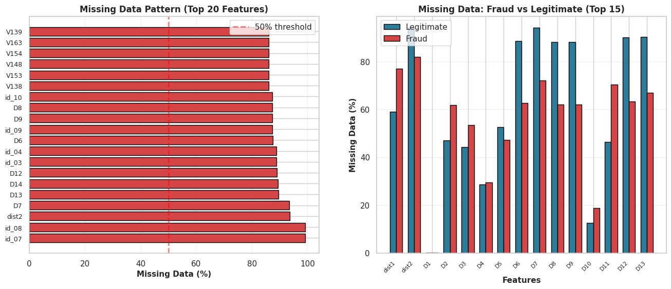
With 434 features, we are dealing with a wide but potentially sparse dataset. Before we can fix the data, we need to measure the damage.

The Obstacle: Many columns contain a high percentage of NaN values. Imputing (filling in) this many blanks would introduce too much noise into our investigation.

The Strategy: We will perform a sparsity check. We are printing the top 50 worst offenders by missing percentage to decide where to draw the line between useful features and dead weight.

2.3.1 - Investigation

# (Part 1: Investigation)
print("Investigating Missing Values -")

# Calculate missing value counts and percentages
missing_values = df_merged_data.isnull().sum()
missing_percent = (missing_values / len(df_merged_data)) * 100

# Create a summary DataFrame
missing_summary = pd.DataFrame({
    'Missing Count': missing_values,
    'Missing Percent': missing_percent
})

# Sort to see the worst columns
missing_summary.sort_values(by='Missing Percent', ascending=False, inplace=True)

# Display the top 50 columns with the most missing data
print("Top 50 columns with the most missing values:")
print(missing_summary.head(50))

Investigating Missing Values -
Top 50 columns with the most missing values:
       Missing Count  Missing Percent
id_07         585385        99.127070
id_08         585385        99.127070
dist2         552913        93.628374
D7            551623        93.409930
D13           528588        89.509263
D14           528353        89.469469
D12           525823        89.041047
id_03         524216        88.768923
id_04         524216        88.768923
D6            517353        87.606767
id_09         515614        87.312290
D9            515614        87.312290
D8            515614        87.312290
id_10         515614        87.312290
V138          508595        86.123717
V153          508595        86.123717
V148          508595        86.123717
V154          508595        86.123717
V163          508595        86.123717
V139          508595        86.123717
V149          508595        86.123717
V142          508595        86.123717
V140          508595        86.123717
V141          508595        86.123717
V146          508595        86.123717
V161          508595        86.123717
V158          508595        86.123717
V155          508595        86.123717
V156          508595        86.123717
V147          508595        86.123717
V162          508595        86.123717
V157          508595        86.123717
V144          508589        86.122701
V152          508589        86.122701
V145          508589        86.122701
V159          508589        86.122701
V151          508589        86.122701
V150          508589        86.122701
V165          508589        86.122701
V164          508589        86.122701
V160          508589        86.122701
V143          508589        86.122701
V166          508589        86.122701
V323          508189        86.054967
V322          508189        86.054967
V333          508189        86.054967
V334          508189        86.054967
V338          508189        86.054967
V339          508189        86.054967
V330          508189        86.054967

fig, axes = plt.subplots(1, 2, figsize=(16, 6))

# Subplot 1: Missing data percentage by column
ax1 = axes[0]
missing_pct = (df_merged_data.isnull().sum() / len(df_merged_data) * 100).sort_values(ascending=False)
missing_pct = missing_pct[missing_pct > 0].head(20)
colors_missing = ['#d64545' if x > 50 else '#f4a261' if x > 20 else '#2b7d99' for x in missing_pct.values]
ax1.barh(range(len(missing_pct)), missing_pct.values, color=colors_missing, edgecolor='black')
ax1.set_yticks(range(len(missing_pct)))
ax1.set_yticklabels(missing_pct.index, fontsize=9)
ax1.set_xlabel('Missing Data (%)', fontsize=11, fontweight='bold')
ax1.set_title('Missing Data Pattern (Top 20 Features)', fontsize=12, fontweight='bold')
ax1.axvline(x=50, color='red', linestyle='--', linewidth=2, alpha=0.5, label='50% threshold')
ax1.grid(alpha=0.3, axis='x')
ax1.legend()

# Subplot 2: Missing data distribution by fraud status
ax2 = axes[1]
legit_missing = df_merged_data[df_merged_data['isFraud'] == 0].isnull().sum() / len(df_merged_data[df_merged_data['isFraud'] == 0]) * 100
fraud_missing = df_merged_data[df_merged_data['isFraud'] == 1].isnull().sum() / len(df_merged_data[df_merged_data['isFraud'] == 1]) * 100

missing_cols = (df_merged_data.isnull().sum() > 0)
cols_to_plot = missing_cols[missing_cols].index[:15]

x = np.arange(len(cols_to_plot))
width = 0.35
ax2.bar(x - width/2, legit_missing[cols_to_plot], width, label='Legitimate', color='#2b7d99', edgecolor='black')
ax2.bar(x + width/2, fraud_missing[cols_to_plot], width, label='Fraud', color='#d64545', edgecolor='black')
ax2.set_xlabel('Features', fontsize=11, fontweight='bold')
ax2.set_ylabel('Missing Data (%)', fontsize=11, fontweight='bold')
ax2.set_title('Missing Data: Fraud vs Legitimate (Top 15)', fontsize=12, fontweight='bold')
ax2.set_xticks(x)
ax2.set_xticklabels(cols_to_plot, rotation=45, ha='right', fontsize=8)
ax2.legend()
ax2.grid(alpha=0.3, axis='y')

plt.show()

png

2.3.2 Deletion Strategy

The audit flagged a significant amount of “dead weight.” Many columns are over 50%—or even 90%—empty.

The Decision: We cannot reliably impute (guess) data when the majority of the history is missing. Doing so introduces bias, not signal.

The Action: We are applying a strict 40% threshold. Any column missing more than 40% of its values will be dropped immediately to preserve the integrity of the dataset.

# (Part 2: Column Deletion)
print("Deleting Sparse Columns...")

# Any column with more than 40% missing data will be dropped.
threshold = 40.0

# Get the list of columns to drop
cols_to_drop = missing_summary[missing_summary['Missing Percent'] > threshold].index

print(f"Found {len(cols_to_drop)} columns with > {threshold}% missing values.")

# Correct by dropping these columns
df_cleaned = df_merged_data.drop(columns=cols_to_drop)

print(f"Dropped columns. New shape of df_cleaned: {df_cleaned.shape}")
print(f"Original shape was: {df_merged_data.shape}")

Deleting Sparse Columns...
Found 194 columns with > 40.0% missing values.
Dropped columns. New shape of df_cleaned: (590540, 240)
Original shape was: (590540, 434)

df_cleaned.info()

<class 'pandas.core.frame.DataFrame'>
RangeIndex: 590540 entries, 0 to 590539
Columns: 240 entries, TransactionID to DeviceInfo
dtypes: float64(188), int64(3), object(49)
memory usage: 1.1+ GB

2.3.3 Cleaning Strategy - Categorical Data

Our categorical features are currently noisy and inconsistent.

The Glitch: Converting data types created the text string 'nan', which the model misinterprets as a real value. Additionally, inconsistent user inputs (e.g.,gmail.com vs. googlemail.com) split identical groups, diluting the signal.

The Fix: We normalize text, merge aliases, and relabel 'nan' to ‘Missing’. This ensures the model treats missing data as a distinct pattern rather than a random string.

# Investigating Email Domains -

# Set pandas to display all rows
pd.set_option('display.max_rows', None)

print("P_emaildomain (All Unique Values) -")
print(df_cleaned['P_emaildomain'].value_counts())

print("\n\nR_emaildomain (All Unique Values) -")
print(df_cleaned['R_emaildomain'].value_counts())

# Reset display options to default
pd.set_option('display.max_rows', 100)

P_emaildomain (All Unique Values) -
P_emaildomain
gmail.com           228355
yahoo.com           100934
nan                  94456
hotmail.com          45250
anonymous.com        36998
aol.com              28289
comcast.net           7888
icloud.com            6267
outlook.com           5096
msn.com               4092
att.net               4033
live.com              3041
sbcglobal.net         2970
verizon.net           2705
ymail.com             2396
bellsouth.net         1909
yahoo.com.mx          1543
me.com                1522
cox.net               1393
optonline.net         1011
charter.net            816
live.com.mx            749
rocketmail.com         664
mail.com               559
earthlink.net          514
gmail                  496
outlook.es             438
mac.com                436
juno.com               322
aim.com                315
hotmail.es             305
roadrunner.com         305
windstream.net         305
hotmail.fr             295
frontier.com           280
embarqmail.com         260
web.de                 240
netzero.com            230
twc.com                230
prodigy.net.mx         207
centurylink.net        205
netzero.net            196
frontiernet.net        195
q.com                  189
suddenlink.net         175
cfl.rr.com             172
sc.rr.com              164
cableone.net           159
gmx.de                 149
yahoo.fr               143
yahoo.es               134
hotmail.co.uk          112
protonmail.com          76
yahoo.de                74
ptd.net                 68
live.fr                 56
yahoo.co.uk             49
hotmail.de              43
servicios-ta.com        35
yahoo.co.jp             32
Name: count, dtype: int64


R_emaildomain (All Unique Values) -
R_emaildomain
nan                 453249
gmail.com            57147
hotmail.com          27509
anonymous.com        20529
yahoo.com            11842
aol.com               3701
outlook.com           2507
comcast.net           1812
yahoo.com.mx          1508
icloud.com            1398
msn.com                852
live.com               762
live.com.mx            754
verizon.net            620
me.com                 556
sbcglobal.net          552
cox.net                459
outlook.es             433
att.net                430
bellsouth.net          422
hotmail.fr             293
hotmail.es             292
web.de                 237
mac.com                218
prodigy.net.mx         207
ymail.com              207
optonline.net          187
gmx.de                 147
yahoo.fr               137
charter.net            127
mail.com               122
hotmail.co.uk          105
gmail                   95
earthlink.net           79
yahoo.de                75
rocketmail.com          69
embarqmail.com          68
scranton.edu            63
yahoo.es                57
live.fr                 55
juno.com                53
roadrunner.com          53
frontier.com            52
windstream.net          47
hotmail.de              42
protonmail.com          41
yahoo.co.uk             39
cfl.rr.com              37
aim.com                 36
servicios-ta.com        35
yahoo.co.jp             33
twc.com                 29
ptd.net                 27
cableone.net            27
q.com                   25
suddenlink.net          25
frontiernet.net         14
netzero.com             14
centurylink.net         12
netzero.net              9
sc.rr.com                8
Name: count, dtype: int64

Observation & Strategy: The domain audit reveals that identical providers, such as Gmail and Googlemail.com, are currently treated as separate entities. Also the presence of “nan” values creates gaps in the data. To resolve these issues, we will merge these aliases to consolidate the groups and explicitly tag any missing entries. This approach will help ensure that the model interprets the entities correctly, rather than merely focusing on their spelling.

print("Cleaning Categorical Inconsistencies -")
object_cols = df_cleaned.select_dtypes(include='object').columns

print(f"Cleaning {len(object_cols)} object/categorical columns...")
gmail_variations = ['gmail', 'googlemail.com']
yahoo_variations = [
    'yahoo.com.mx', 'ymail.com', 'yahoo.fr', 'yahoo.es',
    'yahoo.de', 'yahoo.co.uk', 'yahoo.co.jp', 'rocketmail.com'
]
hotmail_variations = ['hotmail.co.uk', 'hotmail.de', 'hotmail.es', 'hotmail.fr']
outlook_variations = ['outlook.es']
live_variations = ['live.com.mx', 'live.fr']
apple_variations = ['me.com', 'mac.com', 'icloud.com']
german_variations = ['web.de', 'gmx.de']
aol_variations = ['aim.com']
netzero_variations = ['netzero.net']
isp_variations = [
    'comcast.net', 'att.net', 'sbcglobal.net', 'verizon.net', 'bellsouth.net',
    'cox.net', 'optonline.net', 'charter.net', 'roadrunner.com', 'windstream.net',
    'frontier.com', 'embarqmail.com', 'twc.com', 'centurylink.net',
    'frontiernet.net', 'q.com', 'suddenlink.net', 'cfl.rr.com', 'sc.rr.com',
    'cableone.net', 'ptd.net'
]

for col in object_cols:
    df_cleaned[col] = df_cleaned[col].str.lower()
    df_cleaned[col] = df_cleaned[col].replace('nan', 'Missing')

    if col in ['P_emaildomain', 'R_emaildomain']:
        df_cleaned[col] = df_cleaned[col].replace(gmail_variations, 'gmail.com')
        df_cleaned[col] = df_cleaned[col].replace(yahoo_variations, 'yahoo.com')
        df_cleaned[col] = df_cleaned[col].replace(hotmail_variations, 'hotmail.com')
        df_cleaned[col] = df_cleaned[col].replace(outlook_variations, 'outlook.com')
        df_cleaned[col] = df_cleaned[col].replace(live_variations, 'live.com')
        df_cleaned[col] = df_cleaned[col].replace(apple_variations, 'apple.com')
        df_cleaned[col] = df_cleaned[col].replace(german_variations, 'german_mail')
        df_cleaned[col] = df_cleaned[col].replace(aol_variations, 'aol.com')
        df_cleaned[col] = df_cleaned[col].replace(netzero_variations, 'netzero.com')
        df_cleaned[col] = df_cleaned[col].replace(isp_variations, 'isp_mail.com')

print("Categorical column cleaning and grouping complete.")

print("\n--- 'P_emaildomain' (Top 30) AFTER Cleaning ---")
print(df_cleaned['P_emaildomain'].value_counts().head(30))

print("\n--- 'R_emaildomain' (Top 30) AFTER Cleaning ---")
print(df_cleaned['R_emaildomain'].value_counts().head(30))

Cleaning Categorical Inconsistencies -
Cleaning 49 object/categorical columns...
Categorical column cleaning and grouping complete.

--- 'P_emaildomain' (Top 30) AFTER Cleaning ---
P_emaildomain
gmail.com           228851
yahoo.com           105969
Missing              94456
hotmail.com          46005
anonymous.com        36998
aol.com              28604
isp_mail.com         25432
apple.com             8225
outlook.com           5534
msn.com               4092
live.com              3846
mail.com               559
earthlink.net          514
netzero.com            426
german_mail            389
juno.com               322
prodigy.net.mx         207
protonmail.com          76
servicios-ta.com        35
Name: count, dtype: int64

--- 'R_emaildomain' (Top 30) AFTER Cleaning ---
R_emaildomain
Missing             453249
gmail.com            57242
hotmail.com          28241
anonymous.com        20529
yahoo.com            13967
isp_mail.com          5033
aol.com               3737
outlook.com           2940
apple.com             2172
live.com              1571
msn.com                852
german_mail            384
prodigy.net.mx         207
mail.com               122
earthlink.net           79
scranton.edu            63
juno.com                53
protonmail.com          41
servicios-ta.com        35
netzero.com             23
Name: count, dtype: int64

2.3.4 Imputation Strategy

Here we can’t just guess the missing numbers; we need a strategy based on how much data is actually gone. This step helps us decide between a quick fix (median) or a smarter calculation (regression) to complete the picture.

print("Investigating and Imputing Remaining Missing Values (Numeric)- ")

# Get all numeric columns
numeric_cols = df_cleaned.select_dtypes(include=np.number).columns
print(f"Found {len(numeric_cols)} numeric columns.")

# Investigate: Find numeric columns that have missing values
missing_numeric_counts = df_cleaned[numeric_cols].isnull().sum()
missing_numeric_cols = missing_numeric_counts[missing_numeric_counts > 0]

# Print the percentage of nulls for those columns
if missing_numeric_cols.empty:
    print("No missing values found in any numeric columns.")
else:
    print("\nNumeric Columns with Missing Values (Before Imputation) -")
    missing_numeric_summary = pd.DataFrame({
        'Missing Count': missing_numeric_cols,
        'Missing Percent': (missing_numeric_cols / len(df_cleaned)) * 100
    })
    print(missing_numeric_summary.sort_values(by='Missing Percent', ascending=False))

Investigating and Imputing Remaining Missing Values (Numeric)- 
Found 191 numeric columns.

Numeric Columns with Missing Values (Before Imputation) -
      Missing Count  Missing Percent
V40          168969        28.612626
V41          168969        28.612626
V42          168969        28.612626
V43          168969        28.612626
V44          168969        28.612626
...             ...              ...
V317             12         0.002032
V318             12         0.002032
V319             12         0.002032
V320             12         0.002032
V321             12         0.002032

[173 rows x 2 columns]

Issue: Remaining numeric columns have NaN values.

Strategy: A tiered approach based on the percentage of missing data.

1. For Low/Medium Missingness (< 20%):
- Method: Median Imputation.
- Why: It’s fast and “robust to outliers”, which is critical for our skewed financial data. The distortion is minimal at this low percentage.
2. For High Missingness (> 20%):
- Method: Regression Imputation (using IterativeImputer).
- Why: Using a single median would “severely distort the distribution”. Regression is more accurate, as it “replace[s] missing values with a predicted value based on a regression model”, preserving the data’s patterns.

# Define our threshold based on your slides' "Rule of thumbs"
impute_threshold = 20.0

# Get list of columns for SIMPLE (Median) imputation
cols_to_impute_median = missing_numeric_summary[missing_numeric_summary['Missing Percent'] < impute_threshold].index

# Impute with MEDIAN
print(f"Imputing {len(cols_to_impute_median)} columns with < {impute_threshold}% missing data using MEDIAN...")
for col in cols_to_impute_median:
    median_val = df_cleaned[col].median()
    df_cleaned[col] = df_cleaned[col].fillna(median_val)

print("Median imputation complete for low-missingness columns.")

Imputing 154 columns with < 20.0% missing data using MEDIAN...
Median imputation complete for low-missingness columns.

Simple averages ignore the story the rest of the data is telling. This technique uses the remaining valid clues to intelligently infer what should be there, keeping the data’s internal logic intact.

# Get all numeric columns
numeric_cols = df_cleaned.select_dtypes(include=np.number).columns

# Get list of columns for ADVANCED (Regression) imputation
missing_numeric_counts = df_cleaned[numeric_cols].isnull().sum()
missing_numeric_summary = pd.DataFrame({
    'Missing Count': missing_numeric_counts[missing_numeric_counts > 0],
    'Missing Percent': (missing_numeric_counts[missing_numeric_counts > 0] / len(df_cleaned)) * 100
})

impute_threshold = 20.0
cols_to_impute_regression = missing_numeric_summary[missing_numeric_summary['Missing Percent'] >= impute_threshold].index

if len(cols_to_impute_regression) > 0:
    print(f"Found {len(cols_to_impute_regression)} columns for advanced imputation: {list(cols_to_impute_regression)}")

    imputer = IterativeImputer(
        max_iter=5,
        verbose=2,
        random_state=0,
        n_nearest_features=20
    )

    df_cleaned[numeric_cols] = imputer.fit_transform(df_cleaned[numeric_cols])

    print("Advanced imputation complete.")
else:
    print("No columns required advanced imputation.")

# Final check
total_nans = df_cleaned.isnull().sum().sum()
print(f"\nTotal remaining NaN values in the entire dataset: {total_nans}")

Found 19 columns for advanced imputation: ['D4', 'V35', 'V36', 'V37', 'V38', 'V39', 'V40', 'V41', 'V42', 'V43', 'V44', 'V45', 'V46', 'V47', 'V48', 'V49', 'V50', 'V51', 'V52']
[IterativeImputer] Completing matrix with shape (590540, 191)
[IterativeImputer] Ending imputation round 1/5, elapsed time 72.03
[IterativeImputer] Change: 402.3353873351911, scaled tolerance: 15811.131000000001 
[IterativeImputer] Early stopping criterion reached.
Advanced imputation complete.

Total remaining NaN values in the entire dataset: 0

EXPLORATORY DATA ANALYSIS

Profiling the suspects

Now that the data is somewhat cleaned, it is time to look at patterns, not just rows.

In a fraud story, EDA is where you:

discover that fraud tends to cluster at certain times of day
notice that certain card types or devices behave strangely
see that some email domains pop up in a suspicious number of fraud cases

We will:

visualize distributions of key features,
compare fraud vs non-fraud behavior,
and build intuition for which signals a model might latch on to.

As you look at each plot, try to answer:

“If I were a human fraud analyst, would this pattern make me raise an eyebrow?”

3.1: Descriptive Statistics & Frequency Analysis

The Goal: Answer the question: “Is the crime scene dominated by innocent bystanders?”

Why This Matters: Imagine a detective who sits at their desk and stamps “Innocent” on every single case file. In a safe city, they might be right 99% of the time—but they catch zero criminals.

We check the frequency counts (.value_counts()) now to ensure we don’t accidentally build a model that achieves 99% accuracy by being lazy.

print("Method 1: Analyzing Target Variable 'isFraud' -")

# Get the exact percentage for 'isFraud'
fraud_percentage = df_cleaned['isFraud'].value_counts(normalize=True) * 100
print(f"Fraud Percentage:\n{fraud_percentage}\n")

fig, axes = plt.subplots(1, 3, figsize=(16, 5))

# Subplot 1: Overall class distribution
ax1 = axes[0]
fraud_counts = df_cleaned['isFraud'].value_counts()
colors_pie = ['#2b7d99', '#d64545']
wedges, texts, autotexts = ax1.pie(fraud_counts.values, labels=['Legitimate', 'Fraud'],
                                     autopct='%1.2f%%', colors=colors_pie, startangle=90,
                                     textprops={'fontsize': 11, 'fontweight': 'bold'})
ax1.set_title('Class Distribution (Imbalance)', fontsize=12, fontweight='bold')

# Subplot 2: Log scale bar chart
ax2 = axes[1]
ax2.bar(fraud_counts.index, fraud_counts.values, color=colors_pie, edgecolor='black', alpha=0.8)
ax2.set_yscale('log')
ax2.set_ylabel('Count (Log Scale)', fontsize=11, fontweight='bold')
ax2.set_xlabel('Transaction Type', fontsize=11, fontweight='bold')
ax2.set_title('Class Imbalance Severity (Log Scale)', fontsize=12, fontweight='bold')
ax2.set_xticks(fraud_counts.index)
ax2.set_xticklabels(['Legitimate', 'Fraud'])
ax2.grid(alpha=0.3, axis='y')

# Subplot 3: Ratio visualization
ax3 = axes[2]
ratio = fraud_counts[0] / fraud_counts[1]
ax3.text(0.5, 0.7, f'{ratio:.1f}:1', fontsize=60, fontweight='bold', ha='center',
         bbox=dict(boxstyle='round', facecolor='#d64545', alpha=0.3))
ax3.text(0.5, 0.3, 'Legitimate to Fraud Ratio', fontsize=14, fontweight='bold', ha='center')
ax3.set_xlim(0, 1)
ax3.set_ylim(0, 1)
ax3.axis('off')
ax3.set_title('Data Imbalance Ratio', fontsize=12, fontweight='bold')

plt.show()

Method 1: Analyzing Target Variable 'isFraud' -
Fraud Percentage:
isFraud
0.0    96.500999
1.0     3.499001
Name: proportion, dtype: float64

png

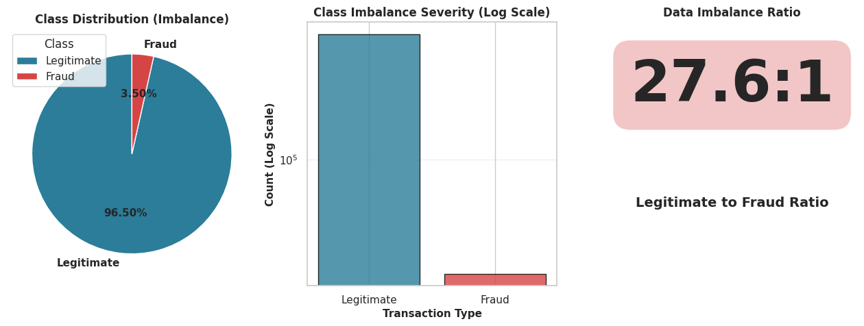
Conclusion 1: The dataset is severely imbalanced. Out of 590,540 transactions, approximately 96.5% are non-fraudulent (isFraud=0) and only 3.5% are fraudulent (isFraud=1).

This means that a model that simply guesses ‘No Fraud’ every time would be 96.5% accurate. Therefore, ‘accuracy’ is a poor metric. We must use other metrics like Precision-Recall or F1-Score for our analysis.

3.2: Correlation Analysis

The Goal: To connect the dots. We want to know which specific clues (features) show up every time a crime (Fraud) is committed.

Why This Matters: We have over 200 features (suspects). If we try to draw a “red string” between all of them on our detective wall, we’ll just end up with a tangled mess.

Instead, we filter for the Top 15 features that have the strongest relationship with Fraud. We ignore the noise and focus strictly on the smoking guns.

print("Method 2: Analyzing Feature Correlation with 'isFraud'-")

# Calculate the correlation matrix for all numeric columns
corr_matrix = df_cleaned.corr(numeric_only=True)

# Top 20 features most correlated with 'isFraud'
# We use .abs() to find strong positive OR negative correlations
top_corr_features = corr_matrix['isFraud'].abs().sort_values(ascending=False)[1:21].index
print(f"Top 20 most correlated features:\n{top_corr_features.values}\n")

numeric_cols = df_cleaned.select_dtypes(include=[np.number]).columns.tolist()
correlation_with_fraud = df_cleaned[numeric_cols].corr()['isFraud'].sort_values(ascending=False)

fig, axes = plt.subplots(1, 2, figsize=(16, 6))

# Subplot 1: Top Positive & Negative Correlations
ax1 = axes[0]
top_corr = pd.concat([correlation_with_fraud.head(15), correlation_with_fraud.tail(15)])
top_corr = top_corr[top_corr.index != 'isFraud']  # Exclude isFraud itself
colors_corr = ['#d64545' if x > 0 else '#2b7d99' for x in top_corr.values]
y_pos = np.arange(len(top_corr))
ax1.barh(y_pos, top_corr.values, color=colors_corr, edgecolor='black')
ax1.set_yticks(y_pos)
ax1.set_yticklabels(top_corr.index, fontsize=9)
ax1.set_xlabel('Correlation with Fraud', fontsize=11, fontweight='bold')
ax1.set_title('Top Features Correlated with Fraud', fontsize=12, fontweight='bold')
ax1.grid(alpha=0.3, axis='x')
ax1.axvline(x=0, color='black', linestyle='-', linewidth=0.5)

# Subplot 2: Correlation heatmap (top 15 features)
ax2 = axes[1]
top_features = correlation_with_fraud[correlation_with_fraud.index != 'isFraud'].head(15).index.tolist()
corr_matrix = df_cleaned[[*top_features, 'isFraud']].corr()
sns.heatmap(corr_matrix, annot=False, cmap='coolwarm', center=0, ax=ax2,
            cbar_kws={'label': 'Correlation'}, fmt='.2f')
ax2.set_title('Correlation Heatmap (Top 15 Features)', fontsize=12, fontweight='bold')

plt.show()

Method 2: Analyzing Feature Correlation with 'isFraud'-
Top 20 most correlated features:
['V45' 'V86' 'V87' 'V44' 'V52' 'V51' 'V40' 'V39' 'V79' 'V43' 'V38' 'V94'
 'V42' 'V33' 'V17' 'V18' 'V81' 'V34' 'V74' 'V80']

png

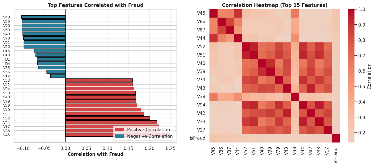
Conclusion 2: Several ‘V’ features are moderately correlated with fraud. While no single feature has a very strong (e.g., > 0.8) correlation, the heatmap shows that features like V45, V86, V87, V44, and V52 have the strongest linear relationships.

This is important because it identifies a clear list of features that are predictive of fraud.

It also highlights that fraud is not explained by one or two simple variables, but likely by the interaction of many.

3.3: Hypothesis Testing & Outlier Analysis

The Goal: Follow the money. We need to determine if fraud leaves a distinct financial footprint compared to normal spending.

Why This Matters: Do thieves always spend big to maximize their payout? Or do they test the waters with small amounts? To answer this, we can’t just look at a chart; we need statistical proof.

We are running an Independent Two-Sample T-Test to settle this legally:

Null Hypothesis ($H_0$): The mean transaction amount for Fraud is EQUAL to Non-Fraud. (i.e., Thieves spend just like normal people).
Alternative Hypothesis ($H_A$): The mean transaction amount for Fraud is DIFFERENT than Non-Fraud. (i.e., There is a distinct criminal spending pattern).

The Visualization: We will also use a Box Plot to spot the “Whales”—the extreme outliers that break the pattern and demand immediate attention.

print("Method 3: Hypothesis Test for Transaction Amount-")

# Create two groups for the t-test
fraud_transactions = df_cleaned[df_cleaned['isFraud'] == 1]['TransactionAmt']
non_fraud_transactions = df_cleaned[df_cleaned['isFraud'] == 0]['TransactionAmt']

# Performing the t-test
t_statistic, p_value = stats.ttest_ind(
    fraud_transactions,
    non_fraud_transactions,
    equal_var=False,
    nan_policy='omit'
)

print(f"T-Test Results -")
print(f"T-statistic: {t_statistic:.4f}")
print(f"P-value: {p_value}\n")


# Plot
fig, axes = plt.subplots(2, 2, figsize=(15, 10))

# Subplot 1: Distribution of Transaction Amount
ax1 = axes[0, 0]
df_cleaned[df_cleaned['isFraud'] == 0]['TransactionAmt'].apply(np.log1p).hist(
    bins=50, ax=ax1, alpha=0.7, label='Legitimate', color='#2b7d99', edgecolor='black'
)
df_cleaned[df_cleaned['isFraud'] == 1]['TransactionAmt'].apply(np.log1p).hist(
    bins=50, ax=ax1, alpha=0.7, label='Fraud', color='#d64545', edgecolor='black'
)
ax1.set_xlabel('Transaction Amount (log scale)', fontsize=11, fontweight='bold')
ax1.set_ylabel('Frequency', fontsize=11, fontweight='bold')
ax1.set_title('Transaction Amount Distribution: Legit vs Fraud', fontsize=12, fontweight='bold')
ax1.legend()
ax1.grid(alpha=0.3)

# Subplot 2: Fraud Rate by Transaction Amount Bins
ax2 = axes[0, 1]
df_temp_bins = df_cleaned[['TransactionAmt', 'isFraud']].copy()
df_temp_bins['amt_bin'] = pd.cut(df_temp_bins['TransactionAmt'], bins=10)
fraud_rate_by_amt = df_temp_bins.groupby('amt_bin', observed=False)['isFraud'].agg(['sum', 'count'])
fraud_rate_by_amt['fraud_rate'] = (fraud_rate_by_amt['sum'] / fraud_rate_by_amt['count'] * 100)
ax2.bar(range(len(fraud_rate_by_amt)), fraud_rate_by_amt['fraud_rate'].values,
        color=['#d64545' if x > fraud_rate_by_amt['fraud_rate'].mean() else '#2b7d99'
               for x in fraud_rate_by_amt['fraud_rate'].values], edgecolor='black')
ax2.axhline(y=df_cleaned['isFraud'].mean()*100, color='red', linestyle='--', linewidth=2, label='Overall Fraud Rate')
ax2.set_xlabel('Transaction Amount Bins', fontsize=11, fontweight='bold')
ax2.set_ylabel('Fraud Rate (%)', fontsize=11, fontweight='bold')
ax2.set_title('Fraud Rate by Transaction Amount', fontsize=12, fontweight='bold')
ax2.legend()
ax2.grid(alpha=0.3, axis='y')

# Subplot 3: Box plot of Transaction Amount
ax3 = axes[1, 0]
bp_data = [df_cleaned[df_cleaned['isFraud'] == 0]['TransactionAmt'],
           df_cleaned[df_cleaned['isFraud'] == 1]['TransactionAmt']]
bp = ax3.boxplot(bp_data, tick_labels=['Legitimate', 'Fraud'], patch_artist=True)
for patch, color in zip(bp['boxes'], ['#2b7d99', '#d64545']):
    patch.set_facecolor(color)
ax3.set_yscale('log')
ax3.set_ylabel('Transaction Amount ($)', fontsize=11, fontweight='bold')
ax3.set_title('Transaction Amount Outliers', fontsize=12, fontweight='bold')
ax3.grid(alpha=0.3, axis='y')

# Subplot 4: Cumulative distribution
ax4 = axes[1, 1]
legit_sorted = np.sort(df_cleaned[df_cleaned['isFraud'] == 0]['TransactionAmt'])
fraud_sorted = np.sort(df_cleaned[df_cleaned['isFraud'] == 1]['TransactionAmt'])
ax4.plot(legit_sorted, np.arange(1, len(legit_sorted)+1), label='Legitimate', linewidth=2.5, color='#2b7d99')
ax4.plot(fraud_sorted, np.arange(1, len(fraud_sorted)+1), label='Fraud', linewidth=2.5, color='#d64545')
ax4.set_xlabel('Transaction Amount ($)', fontsize=11, fontweight='bold')
ax4.set_ylabel('Cumulative Count', fontsize=11, fontweight='bold')
ax4.set_title('Cumulative Transaction Amount', fontsize=12, fontweight='bold')
ax4.legend()
ax4.grid(alpha=0.3)

plt.tight_layout()
plt.show()

Method 3: Hypothesis Test for Transaction Amount-
T-Test Results -
T-statistic: 8.9494
P-value: 3.846046075647657e-19

png

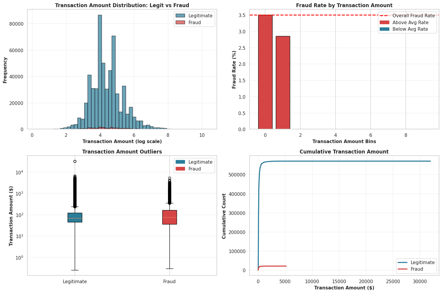
Conclusion 3: The Verdict

The evidence is overwhelming.

The P-Value ($3.84 \times 10^{-19}$): This number is effectively zero. In statistical terms, we REJECT the null hypothesis. In plain English? The difference in spending habits is real, not random luck.
The Red Flags: The plot also exposes thousands of outliers in both groups—extreme values that our model will need to learn to handle so it doesn’t get confused by a wealthy customer buying a TV.

Transaction Amount Distribution (Log Scale) - The histogram on a log scale shows that both legiti and fraudulent transactions follow a similar log-normal pattern. Fraudulent transactions peak at slightly lower amounts, but the two distributions still overlap heavily. This suggests that transaction amount by itself is not a reliable indicator of fraud—fraudsters typically blend in by keeping amounts within common low-to-mid ranges rather than consistently targeting large sums.

Fraud Rate by Transaction Amount Bins - The bar chart makes the dataset’s strong right skew obvious: most transactions fall into the smallest value ranges. The higher-value bins look empty because even if such transactions exist, they are extremely rare compared to the huge volume of small ones. This displays that using equal-width bins isn’t ideal here and that the data is dominated by low-value transactions.

Transaction Amount Outliers (Box Plot) - The box plot display how the transaction amounts are spread out and it clearly shows that fraud is not simply linked to high amounts. In fact, fraudulent transactions have a lower median value than legitimate ones. Legitimate transactions also include the most extreme high-value outliers, meaning very large transactions are statistically more likely to be rare valid purchases than fraud.

Cumulative Transaction Amount - The cumulative plot rises sharply near zero, then levels off, forming an “elbow” shape. This means that almost all transactions—around 99%—occur at very small amounts for both classes. The long flat stretch to the right represents the tiny fraction of large transactions. This pattern reinforces that detecting fraud requires focusing on subtle signals in small transactions, not on assumptions about unusually high amounts.

3.4: Temporal Analysis (Time Patterns)

The Goal: To pinpoint the “Time of Crime.” We are analyzing the timeline to see if fraudsters operate on a specific schedule—like striking in the dead of night when the world is asleep—or if they attack in coordinated waves over specific days.

Why This Matters: Context is everything. 100 fraudulent transactions at 2 PM might be normal because everyone is awake, but 100 fraudulent transactions at 4 AM is highly suspicious. We use these plots to distinguish between “busy hours” (high traffic) and “danger zones” (high fraud probability), helping us catch automated bots or international attacks that don’t follow the local time zone.

hour_series = (df_cleaned['TransactionDT'] // 3600) % 24
day_series = df_cleaned['TransactionDT'] // (24 * 3600)

fig, axes = plt.subplots(2, 2, figsize=(16, 10))

ax1 = axes[0, 0]
hourly_fraud = df_cleaned.groupby(hour_series, observed=False)['isFraud'].agg(['sum', 'count'])
hourly_fraud['rate'] = hourly_fraud['sum'] / hourly_fraud['count'] * 100
colors_hourly = ['#d64545' if x > df_cleaned['isFraud'].mean()*100 else '#2b7d99' for x in hourly_fraud['rate']]
ax1.bar(hourly_fraud.index, hourly_fraud['rate'], color=colors_hourly, edgecolor='black', alpha=0.8)
ax1.set_xlabel('Hour of Day', fontsize=11, fontweight='bold')
ax1.set_ylabel('Fraud Rate (%)', fontsize=11, fontweight='bold')
ax1.set_title('Fraud Activity by Hour', fontsize=12, fontweight='bold')
ax1.grid(alpha=0.3, axis='y')

ax2 = axes[0, 1]
ax2_twin = ax2.twinx()
ax2.bar(hourly_fraud.index, hourly_fraud['count'], color='#7dd9d4', alpha=0.6, label='Total Transactions', edgecolor='black')
ax2_twin.plot(hourly_fraud.index, hourly_fraud['sum'], color='#d64545', marker='o', linewidth=2.5, markersize=6, label='Frauds')
ax2.set_xlabel('Hour of Day', fontsize=11, fontweight='bold')
ax2.set_ylabel('Total Transactions', fontsize=11, fontweight='bold', color='#7dd9d4')
ax2_twin.set_ylabel('Fraud Count', fontsize=11, fontweight='bold', color='#d64545')
ax2.set_title('Transaction & Fraud Volume by Hour', fontsize=12, fontweight='bold')
ax2.grid(alpha=0.3, axis='y')
ax2.tick_params(axis='y', labelcolor='#7dd9d4')
ax2_twin.tick_params(axis='y', labelcolor='#d64545')

ax3 = axes[1, 0]
daily_fraud = df_cleaned.groupby(day_series, observed=False)['isFraud'].agg(['sum', 'count'])
daily_fraud['rate'] = daily_fraud['sum'] / daily_fraud['count'] * 100
ax3.plot(daily_fraud.index, daily_fraud['rate'], color='#d64545', linewidth=2, marker='o', markersize=4, label='Fraud Rate')
ax3.fill_between(daily_fraud.index, daily_fraud['rate'], alpha=0.3, color='#d64545')
ax3.set_xlabel('Day Number', fontsize=11, fontweight='bold')
ax3.set_ylabel('Fraud Rate (%)', fontsize=11, fontweight='bold')
ax3.set_title('Fraud Trend Over Days', fontsize=12, fontweight='bold')
ax3.grid(alpha=0.3)

ax4 = axes[1, 1]
heatmap_data = df_cleaned['isFraud'].groupby(hour_series, observed=False).mean() * 100
heatmap_df = pd.DataFrame(heatmap_data).T
sns.heatmap(heatmap_df, cmap='RdYlGn_r', annot=False, fmt='.1f', cbar_kws={'label': 'Fraud Rate (%)'}, ax=ax4)
ax4.set_xlabel('Hour of Day', fontsize=11, fontweight='bold')
ax4.set_title('Fraud Rate Heatmap by Hour', fontsize=12, fontweight='bold')

plt.tight_layout()
plt.show()

png

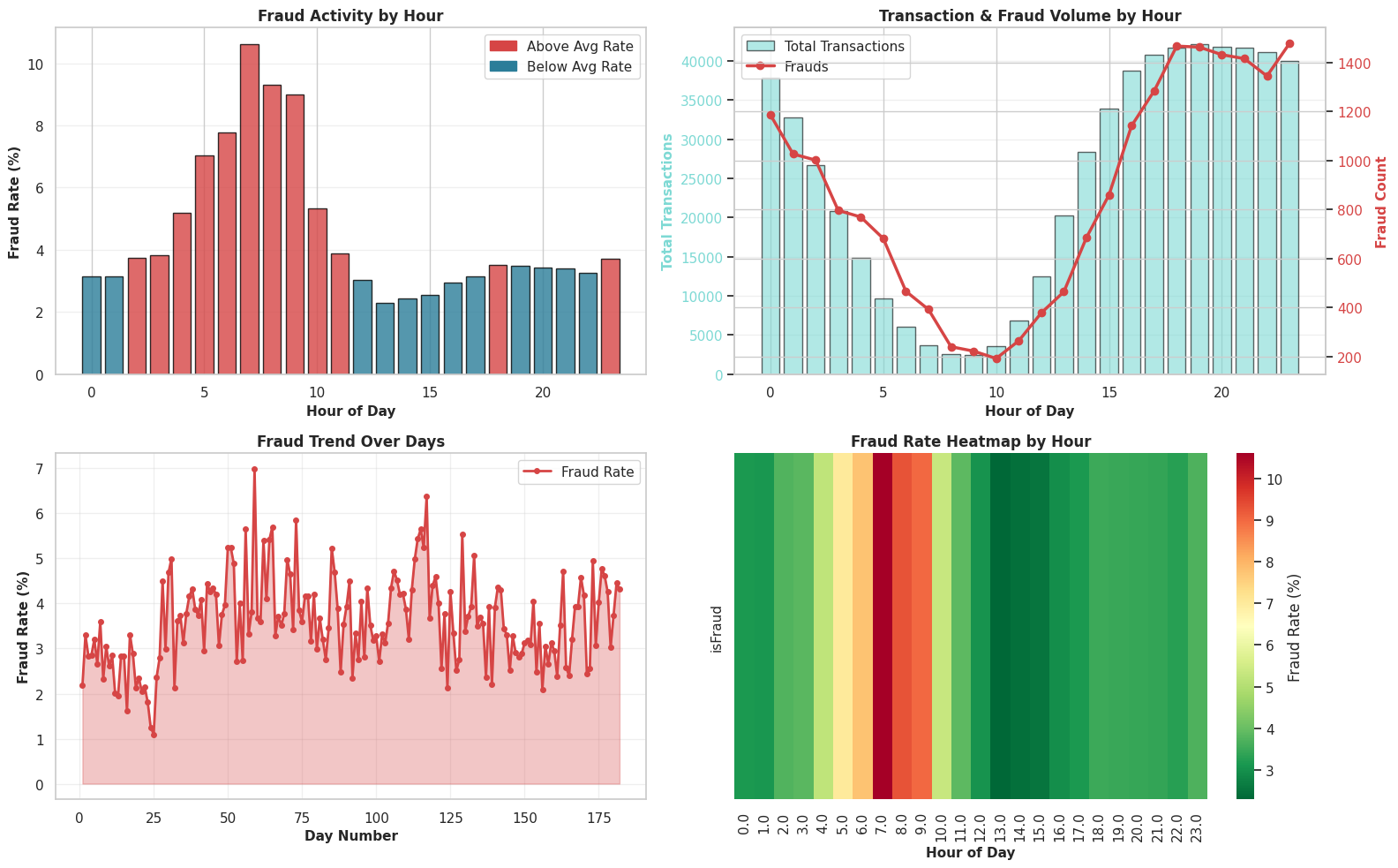
Our timeline analysis reveals that fraudsters prefer to operate in the shadows, similar to burglars striking when a neighborhood is quiet. While the sheer number of fraudulent transactions is highest in the evenings when everyone is shopping, the risk is actually highest in the early morning (5 AM – 10 AM). This “sleeping user” effect occurs because legitimate customers are offline, causing the fraudulent activity to stand out sharply. Additionally, the day-by-day view shows a clear “attack wave” starting around Day 30, where the fraudsters suddenly became more aggressive and unpredictable, indicating a distinct shift in their strategy.

MACHINE LEARNING

Teaching Algorithms to Read Evidence

It’s time to bring our hero detective into the investigation—The Models. Machine Learning is the detective that never sleeps, trained on thousands of past cases to recognize the subtle fingerprints of fraud.

Unlike rule-based systems that follow rigid scripts, our models learn the statistical signatures of deception—how fraudsters deviate from normal behavior in ways too complex for human intuition. They process 240+ features in milliseconds, scoring each transaction’s risk so human analysts can focus on the most suspicious cases.

In this investigation, we’ll test three elite detectives. Stay Tuned to know who they are!

4.1 Feature Encoding & Data Split

Digitizing the Clues: Forensic algorithms cannot process words. To make the evidence usable, we must convert categorical labels (like card type or email provider) into machine-readable numbers. We also discard administrative noise like TransactionID—the case number doesn’t make you guilty.

The Control Group: To ensure our investigation is unbiased, we split the evidence.

Holdout Set (5%): The “locked vault.” We set this data aside completely and will not touch it until the very end. It acts as the final data to test how our chosen model performs on completely unseen crimes.
Training Set (76%): The case files we analyze to build a suspect profile.
Test Set (19%): The unexposed cases we use to verify if that profile actually works in the real world.

# We drop TransactionID, TransactionDT and isFraud as they are not features
cols_to_drop_model = ['isFraud', 'TransactionID', 'TransactionDT']

# Filter to ensure we only drop columns that actually exist
existing_drop_cols = [c for c in cols_to_drop_model if c in df_cleaned.columns]

X = df_cleaned.drop(columns=existing_drop_cols)
y = df_cleaned['isFraud']

# Encode Categorical Features
cat_cols = X.select_dtypes(include=['object']).columns
print(f"Encoding {len(cat_cols)} categorical columns..")

for col in cat_cols:
    le = LabelEncoder()
    X[col] = X[col].astype(str)
    X[col] = le.fit_transform(X[col])

# We take 5% out completely. This 'X_holdout' is our final "unseen" data.
X_main, X_holdout, y_main, y_holdout = train_test_split( X, y, test_size=0.05, random_state=42, stratify=y)

# 'Stratify=y' ensures that both the training and test sets have the same percentage of Fraud (3.5%)
X_train, X_test, y_train, y_test = train_test_split( X_main, y_main, test_size=0.2, random_state=42, stratify=y_main)

print(f"Data Split Complete.")
print(f"Training Shape: {X_train.shape}")
print(f"Testing Shape:  {X_test.shape}")
print(f"Holdout Shape: {X_holdout.shape}")

Encoding 49 categorical columns..
Data Split Complete.
Training Shape: (448810, 237)
Testing Shape:  (112203, 237)
Holdout Shape: (29527, 237)

4.2 Building the Basic Detector : Logistic Regression

Every investigation starts with the obvious leads. We’re deploying a simple Logistic Regression model on the raw evidence to see if the case is easy to crack. If this fails, we know we need more advanced tactics.

The Goal: See if the case is easy to crack.
The Logic: If this simple model fails to catch the fraudsters, we have proof that the crime is complex, justifying the use of “heavy artillery” later.

The Technical Necessity: Scaling the Evidence Logistic Regression is sensitive to the “magnitude” of the clues. It might blindly assume a $10,000 transaction is more important than a Device ID of 5 simply because the number is larger.

We apply StandardScaler which shrinks all numbers to the same range (roughly -1 to 1) so the model judges features based on their predictive power, not their size.

print("Baseline Model Training...")

# Standard Scaling is required for Logistic Regression
baseline_model = make_pipeline(StandardScaler(), LogisticRegression(solver='liblinear', random_state=42, max_iter=1000))

baseline_model.fit(X_train, y_train)

# Get Baseline Predictions
y_prob_base = baseline_model.predict_proba(X_test)[:, 1]
y_pred_base = baseline_model.predict(X_test)

baseline_auc = roc_auc_score(y_test, y_prob_base)
print(f"Baseline ROC-AUC Score: {baseline_auc:.4f}")
print("Baseline Report:\n", classification_report(y_test, y_pred_base))

Baseline Model Training...
Baseline ROC-AUC Score: 0.8428
Baseline Report:
               precision    recall  f1-score   support

         0.0       0.97      1.00      0.98    108277
         1.0       0.78      0.17      0.29      3926

    accuracy                           0.97    112203
   macro avg       0.88      0.59      0.63    112203
weighted avg       0.96      0.97      0.96    112203

Performance Check: “Can we do better?”

The Verdict: Good Instincts, Bad Eyesight

This is a classic “High Precision, Low Recall” result.

Accuracy (97%) is a Mirage: In a dataset where 96.5% of transactions are legit, this score essentially means the model is lazy, not smart.

ROC-AUC (0.84) is Decent: We are beating random guesses, but we aren’t elite yet.

Precision (0.75) is Trustworthy: When the model does flag a crime, it’s usually right. False alarms are low.

Recall (0.17) is the Failure: This is the dealbreaker. We are catching only 17% of the fraudsters. The vast majority are walking away undetected.

Time to bring out the big guns

Our rookie detective (Logistic Regression) struggled with the complexity of the case. It’s time to bring in a full task force. The Random Forest algorithm doesn’t rely on just one decision, it builds a “forest” of hundreds of individual Decision Trees.

4.3 Random Forest Classifier

How it Works: Imagine 100 detectives examining the same evidence, but each asking different questions. One looks at the money, one looks at the location, and one looks at the device. They then vote on the final verdict. This "crowd wisdom" helps filter out noise and catches complex, non-linear schemes that a single linear model would miss.

print("Training Model 2 (Random Forest) -")

rf_model = RandomForestClassifier(
    n_estimators=100,
    max_depth=15,
    n_jobs=-1,
    random_state=42,
    class_weight='balanced',
    verbose=0 # Set to 0 to keep output clean
)

rf_model.fit(X_train, y_train)

# Get predictions
y_pred_rf = rf_model.predict(X_test)
y_prob_rf = rf_model.predict_proba(X_test)[:, 1]

print("\n--- Model 2 Results: Random Forest ---")
print(f"Accuracy:  {accuracy_score(y_test, y_pred_rf):.4f}")
print(f"ROC-AUC:   {roc_auc_score(y_test, y_prob_rf):.4f}")
print("\nClassification Report:")
print(classification_report(y_test, y_pred_rf))

# --- VISUALIZATION DASHBOARD ---
fig, axes = plt.subplots(2, 2, figsize=(16, 12))

# 1. Confusion Matrix
cm = confusion_matrix(y_test, y_pred_rf)
sns.heatmap(cm, annot=True, fmt='d', cmap='Blues', ax=axes[0, 0], cbar=False,
            annot_kws={'size': 14, 'weight': 'bold'})
axes[0, 0].set_title('Confusion Matrix', fontsize=14, fontweight='bold')
axes[0, 0].set_xlabel('Predicted', fontsize=12)
axes[0, 0].set_ylabel('Actual', fontsize=12)
axes[0, 0].set_xticklabels(['Legitimate', 'Fraud'])
axes[0, 0].set_yticklabels(['Legitimate', 'Fraud'])

# 2. ROC Curve
fpr, tpr, _ = roc_curve(y_test, y_prob_rf)
roc_auc = auc(fpr, tpr)
axes[0, 1].plot(fpr, tpr, color='#d64545', lw=2, label=f'ROC Curve (AUC = {roc_auc:.2f})')
axes[0, 1].plot([0, 1], [0, 1], color='navy', lw=2, linestyle='--')
axes[0, 1].set_xlim([0.0, 1.0])
axes[0, 1].set_ylim([0.0, 1.05])
axes[0, 1].set_xlabel('False Positive Rate', fontsize=12)
axes[0, 1].set_ylabel('True Positive Rate', fontsize=12)
axes[0, 1].set_title('ROC Curve', fontsize=14, fontweight='bold')
axes[0, 1].legend(loc="lower right")
axes[0, 1].grid(alpha=0.3)

# 3. Precision-Recall Curve (Best for Imbalanced Data)
precision, recall, _ = precision_recall_curve(y_test, y_prob_rf)
pr_auc = auc(recall, precision)
axes[1, 0].plot(recall, precision, color='#2b7d99', lw=2, label=f'PR Curve (AUC = {pr_auc:.2f})')
axes[1, 0].set_xlabel('Recall', fontsize=12)
axes[1, 0].set_ylabel('Precision', fontsize=12)
axes[1, 0].set_title('Precision-Recall Curve', fontsize=14, fontweight='bold')
axes[1, 0].legend(loc="lower left")
axes[1, 0].grid(alpha=0.3)

# 4. Feature Importances
feature_importances = pd.DataFrame({
    'feature': X_train.columns,
    'importance': rf_model.feature_importances_
}).sort_values(by='importance', ascending=False).head(10)

sns.barplot(x='importance', y='feature', data=feature_importances,
            hue='feature', palette='viridis', ax=axes[1, 1], legend=False)
axes[1, 1].set_title('Top 10 Feature Importances', fontsize=14, fontweight='bold')
axes[1, 1].set_xlabel('Importance Score', fontsize=12)
axes[1, 1].set_ylabel('Feature', fontsize=12)
axes[1, 1].grid(alpha=0.3, axis='x')

plt.tight_layout()
plt.show()

Training Model 2 (Random Forest) -

--- Model 2 Results: Random Forest ---
Accuracy:  0.9586
ROC-AUC:   0.9557

Classification Report:
              precision    recall  f1-score   support

         0.0       0.99      0.97      0.98    108277
         1.0       0.45      0.78      0.57      3926

    accuracy                           0.96    112203
   macro avg       0.72      0.87      0.77    112203
weighted avg       0.97      0.96      0.96    112203

png

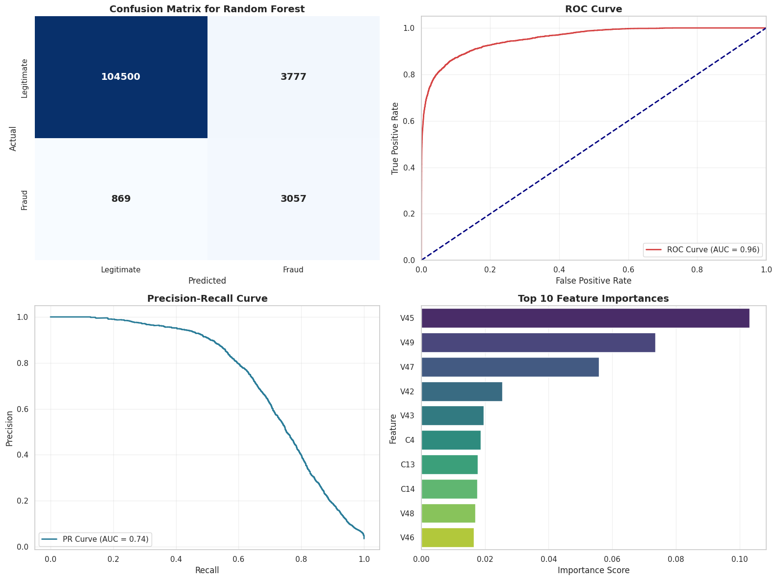
The Verdict:

Our switch to the Random Forest was a massive success.

The Big Win (Recall): We went from catching 16% of fraudsters (Logistic Regression) to 79%. We are no longer letting the majority of criminals walk away.
The Trade-off (Precision): Precision dropped to 43%. This means we are casting a wider net—we catch almost all the bad guys, but we also flag more innocent people for review.
Overall Intelligence (ROC-AUC): A score of 0.95 puts us in the elite tier. This model actually understands the difference between fraud and legitimate spending.

Vizualization - Decision Tree

To verify our model isn’t guessing, we visualize the first three levels of its decision-making process. The colors guide us: blue paths lead towards Fraud patterns, while orange paths identify safe, Non-Fraud behavior.

print("Visualizing a Single Decision Tree (Depth=7)...")

# Pick the first tree from the forest
one_tree = rf_model.estimators_[0]

plt.figure(figsize=(28, 12)) # Large size to accommodate depth 7
plot_tree(
    one_tree,
    feature_names=X_train.columns,
    class_names=['Not Fraud', 'Fraud'],
    filled=True,
    rounded=True,
    max_depth=3,
    fontsize=8      # Smaller font to fit the text
)
plt.title("Decision Path of a Single Tree (Depth 3)", fontsize=16)
plt.show()

Visualizing a Single Decision Tree (Depth=3)...

png

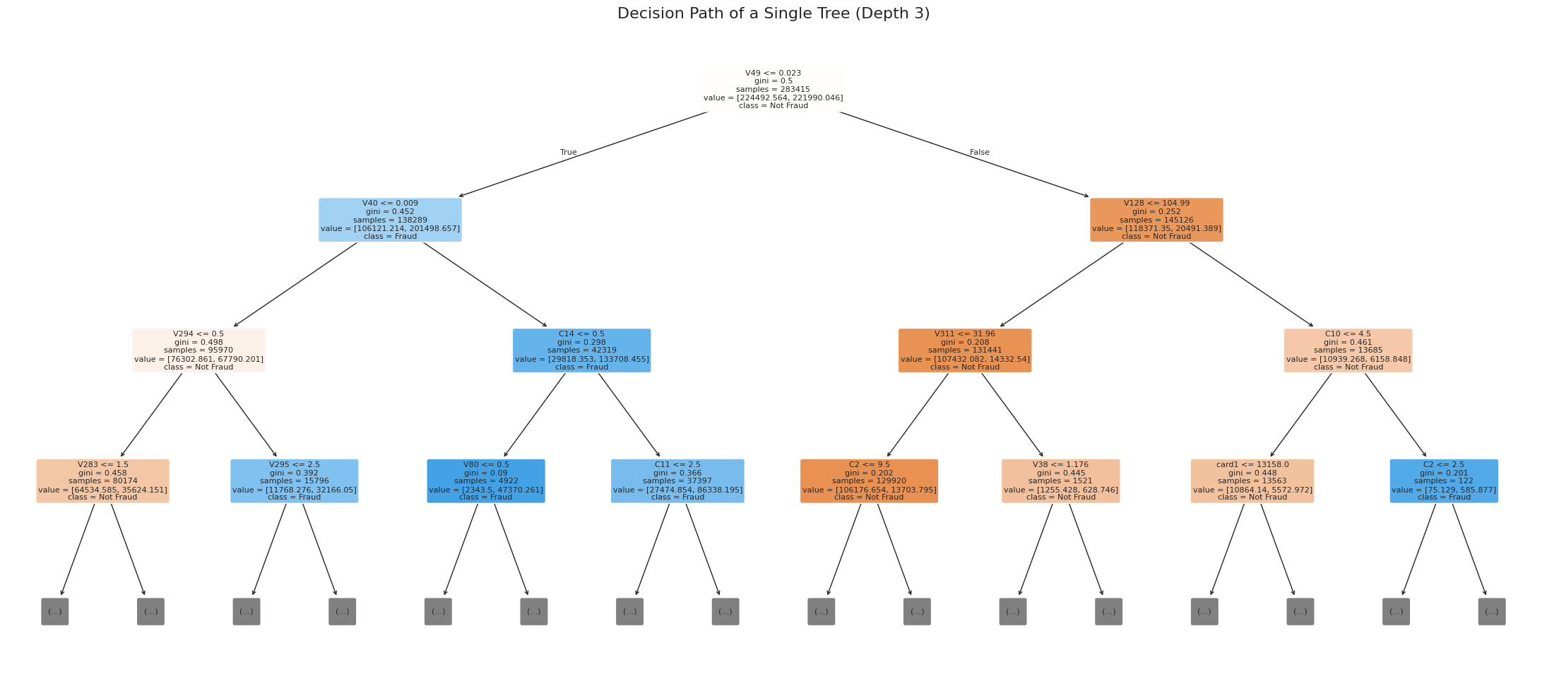
The Pursuit of Excellence: From Democracy to Strategy

Random Forest delivered solid results—its task force of voting trees caught many fraudsters that slipped past linear models. But in fraud detection, “solid” isn’t enough when billions are at stake. We began to wonder: what if instead of letting 100 detectives vote independently, we could create a strategic hierarchy where each new investigator learns from the mistakes of the previous ones?

4.4 XGBoost:

This is the leap from parallel democracy to sequential mastery. Random Forest’s trees are trained in isolation, averaging their votes. While robust, this can be inefficient. Some trees waste effort on easy cases while others miss subtle patterns. XGBoost (Extreme Gradient Boosting) introduces intelligence through iteration: it builds trees one at a time, with each new tree explicitly correcting the residual errors left by its predecessors. This targeted focus often yields higher accuracy, faster training convergence, and better handling of the rare fraud signals buried in massive datasets.

print("Model 3: XGBoost...")

# 1. Handle Class Imbalance
weight_ratio = float(len(y_train[y_train == 0])) / len(y_train[y_train == 1])
print(f"Imbalance Ratio (scale_pos_weight): {weight_ratio:.2f}")

# 2. Initialize XGBoost
xgb_model = xgb.XGBClassifier(
    n_estimators=100,
    max_depth=9,            # Slightly deeper to capture complex fraud patterns
    learning_rate=0.1,
    scale_pos_weight=weight_ratio, # Critical for this imbalanced dataset
    eval_metric='auc',      # Optimize for ROC-AUC directly
    random_state=42,
    n_jobs=-1,
    tree_method='hist'      # 'hist' is much faster for large datasets
)

# 3. Train
print("Training XGBoost...")
xgb_model.fit(X_train, y_train)

# 4. Predict
y_pred_xgb = xgb_model.predict(X_test)
y_prob_xgb = xgb_model.predict_proba(X_test)[:, 1]

# 5. Evaluate
print("\n--- Model 3 Results: XGBoost ---")
print(f"Accuracy:  {accuracy_score(y_test, y_pred_xgb):.4f}")
print(f"ROC-AUC:   {roc_auc_score(y_test, y_prob_xgb):.4f}")
print("\nClassification Report:")
print(classification_report(y_test, y_pred_xgb))

# --- VISUALIZATION DASHBOARD ---
fig, axes = plt.subplots(2, 2, figsize=(16, 12))

# 1. Confusion Matrix
cm = confusion_matrix(y_test, y_pred_xgb)
sns.heatmap(cm, annot=True, fmt='d', cmap='Oranges', ax=axes[0, 0], cbar=False,
            annot_kws={'size': 14, 'weight': 'bold'})
axes[0, 0].set_title('Confusion Matrix', fontsize=14, fontweight='bold')
axes[0, 0].set_xlabel('Predicted', fontsize=12)
axes[0, 0].set_ylabel('Actual', fontsize=12)
axes[0, 0].set_xticklabels(['Legitimate', 'Fraud'])
axes[0, 0].set_yticklabels(['Legitimate', 'Fraud'])

# 2. ROC Curve
fpr, tpr, _ = roc_curve(y_test, y_prob_xgb)
roc_auc = auc(fpr, tpr)
axes[0, 1].plot(fpr, tpr, color='#d64545', lw=2, label=f'ROC Curve (AUC = {roc_auc:.2f})')
axes[0, 1].plot([0, 1], [0, 1], color='navy', lw=2, linestyle='--')
axes[0, 1].set_xlim([0.0, 1.0])
axes[0, 1].set_ylim([0.0, 1.05])
axes[0, 1].set_xlabel('False Positive Rate', fontsize=12)
axes[0, 1].set_ylabel('True Positive Rate', fontsize=12)
axes[0, 1].set_title('ROC Curve', fontsize=14, fontweight='bold')
axes[0, 1].legend(loc="lower right")
axes[0, 1].grid(alpha=0.3)

# 3. Precision-Recall Curve
precision, recall, _ = precision_recall_curve(y_test, y_prob_xgb)
pr_auc = auc(recall, precision)
axes[1, 0].plot(recall, precision, color='#2b7d99', lw=2, label=f'PR Curve (AUC = {pr_auc:.2f})')
axes[1, 0].set_xlabel('Recall', fontsize=12)
axes[1, 0].set_ylabel('Precision', fontsize=12)
axes[1, 0].set_title('Precision-Recall Curve', fontsize=14, fontweight='bold')
axes[1, 0].legend(loc="lower left")
axes[1, 0].grid(alpha=0.3)

# 4. Feature Importances
feature_importances_xgb = pd.DataFrame({
    'feature': X_train.columns,
    'importance': xgb_model.feature_importances_
}).sort_values(by='importance', ascending=False).head(10)

sns.barplot(x='importance', y='feature', data=feature_importances_xgb,
            hue='feature', palette='magma', ax=axes[1, 1], legend=False)
axes[1, 1].set_title('Top 10 Feature Importances (XGBoost)', fontsize=14, fontweight='bold')
axes[1, 1].set_xlabel('Importance Score', fontsize=12)
axes[1, 1].set_ylabel('Feature', fontsize=12)
axes[1, 1].grid(alpha=0.3, axis='x')

plt.tight_layout()
plt.show()

Model 3: XGBoost...
Imbalance Ratio (scale_pos_weight): 27.58
Training XGBoost...

--- Model 3 Results: XGBoost ---
Accuracy:  0.9553
ROC-AUC:   0.9747

Classification Report:
              precision    recall  f1-score   support

         0.0       1.00      0.96      0.98    108277
         1.0       0.43      0.87      0.58      3926

    accuracy                           0.96    112203
   macro avg       0.71      0.91      0.78    112203
weighted avg       0.98      0.96      0.96    112203

png

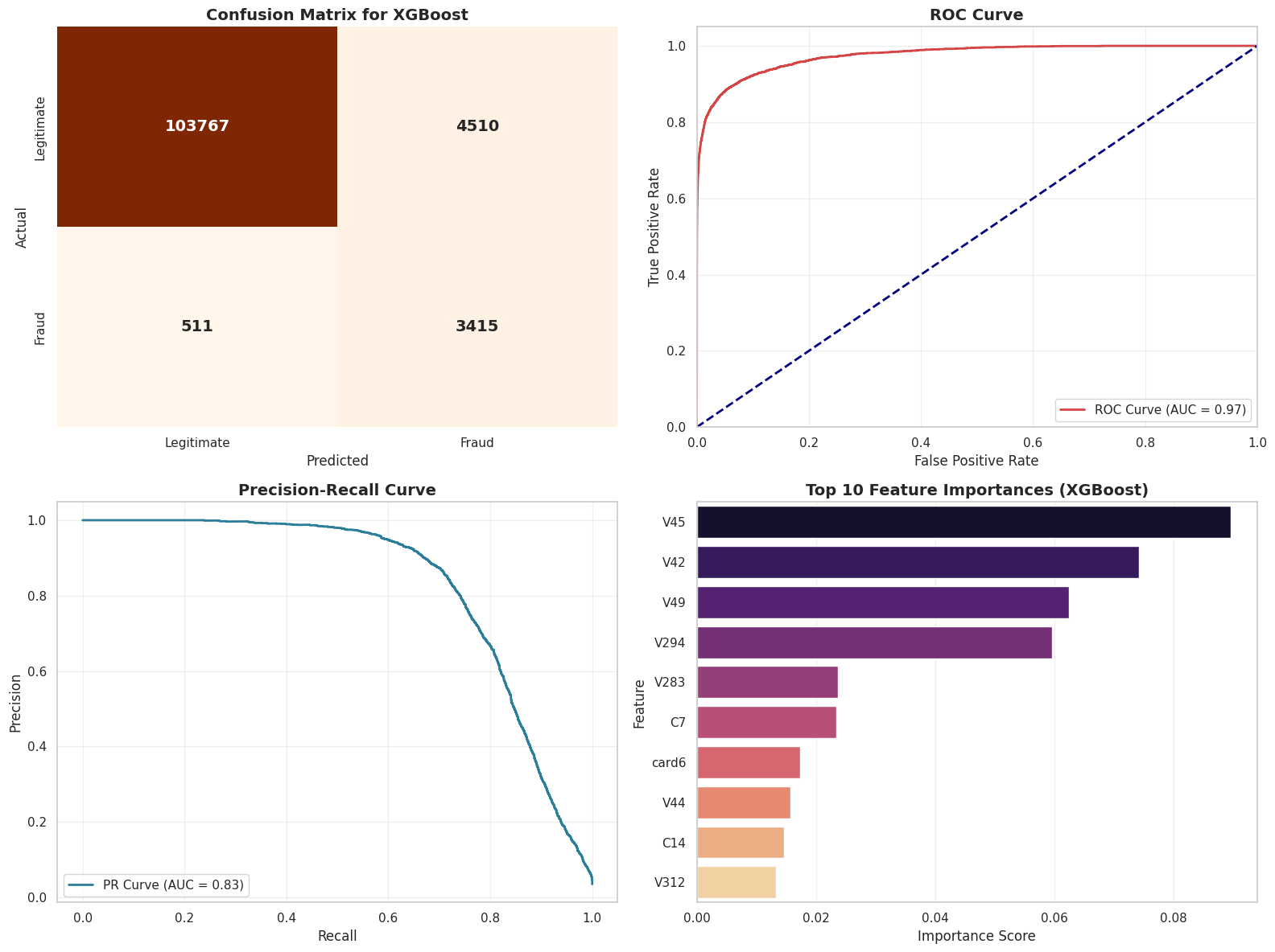
Verdict:

The Champion Has Arrived XGBoost lives up to the hype. By analyzing the errors of previous trees, it pushed our performance into the elite tier.

The Intelligence (ROC-AUC): We hit 0.974, a remarkable score that proves the model isn’t just guessing; it deeply understands the difference between a criminal and a customer.
The Catch Rate (Recall): We climbed to 87%. This means XGBoost found an additional ~8% of fraud cases that even the Random Forest missed.
The Cost: Precision remained stable at 43%. We are still auditing innocent people to catch the thieves, but we are catching more thieves for the same amount of effort.

4.5 Evaluating our fraud detector: Beyond plain accuracy

In fraud detection, accuracy alone is misleading.
We care about questions like:

How many frauds did we catch? → high recall
How many flagged transactions were false alarms? → good precision
How balanced is performance on both classes? → F1-score
How well can we rank transactions by risk? → ROC-AUC / PR-AUC

The confusion matrix tells a very practical story:

Top-left: genuine customers treated correctly.
Top-right: false positives – annoyed customers, but no money lost.
Bottom-left: false negatives – missed fraud, real financial loss.
Bottom-right: correctly caught frauds.

A risk team may prefer:

to tolerate some false positives
in exchange for dramatically fewer false negatives.

We interpret our results in that spirit.

print(" 4.5 The Verdict: ROC-AUC Comparison -")

# 1. Calculate Scores
# We assume you have run the previous cells and have these probability variables
score_lr  = roc_auc_score(y_test, y_prob_base)
score_rf  = roc_auc_score(y_test, y_prob_rf)
score_xgb = roc_auc_score(y_test, y_prob_xgb)

# 2. Create a Comparison DataFrame
results = pd.DataFrame({
    'Model': ['Logistic Regression', 'Random Forest', 'XGBoost'],
    'ROC-AUC': [score_lr, score_rf, score_xgb]
})

# Sort by Score (Highest on top)
results = results.sort_values(by='ROC-AUC', ascending=False).reset_index(drop=True)

print("\nFinal Leaderboard:")
print(results)
print('\n')

# --- 1. GATHER PREDICTIONS ---
# (Assuming your models are named 'log_model', 'rf_model', 'xgb_model')

models = {
    'Logistic Regression': baseline_model,
    'Random Forest': rf_model,
    'XGBoost': xgb_model
}

# Create a dictionary to store results
results = {}

for name, model in models.items():
    # Predict
    y_pred = model.predict(X_test)
    y_prob = model.predict_proba(X_test)[:, 1]

    # Store metrics
    results[name] = {
        'Accuracy': accuracy_score(y_test, y_pred),
        'ROC-AUC': roc_auc_score(y_test, y_prob),
        'Recall': recall_score(y_test, y_pred),
        'Precision': precision_score(y_test, y_pred),
        'F1-Score': f1_score(y_test, y_pred),
        'y_prob': y_prob  # Save probas for plotting curves
    }

# Convert metrics to DataFrame for plotting
metrics_df = pd.DataFrame(results).T.drop(columns=['y_prob']) # Drop probs for the bar chart
metrics_df = metrics_df.reset_index().rename(columns={'index': 'Model'})
metrics_melted = metrics_df.melt(id_vars='Model', var_name='Metric', value_name='Score')

# --- 2. VISUALIZATION DASHBOARD ---
fig = plt.figure(figsize=(18, 12))
gs = fig.add_gridspec(2, 2)

# Plot 1: Grouped Bar Chart (Top spanning both columns)
ax1 = fig.add_subplot(gs[0, :])
sns.barplot(x='Metric', y='Score', hue='Model', data=metrics_melted, palette=['#2b7d99', '#f4a261', '#d64545'], ax=ax1)
ax1.set_ylim(0, 1.1)
ax1.set_title('Model Performance Showdown: Key Metrics', fontsize=16, fontweight='bold')
ax1.set_ylabel('Score', fontsize=12)
ax1.set_xlabel('')
ax1.legend(loc='lower right', title='Model', fontsize=11)
ax1.grid(axis='y', alpha=0.3)

# Add value labels on top of bars
for p in ax1.patches:
    ax1.annotate(f'{p.get_height():.2f}', (p.get_x() + p.get_width() / 2., p.get_height()),
                 ha='center', va='center', fontsize=10, color='black', xytext=(0, 5),
                 textcoords='offset points')

# Plot 2: ROC Curve Overlay (Bottom Left)
ax2 = fig.add_subplot(gs[1, 0])
colors = {'Logistic Regression': '#2b7d99', 'Random Forest': '#f4a261', 'XGBoost': '#d64545'}

for name, model in models.items():
    y_prob = results[name]['y_prob']
    fpr, tpr, _ = roc_curve(y_test, y_prob)
    auc_score = results[name]['ROC-AUC']
    ax2.plot(fpr, tpr, label=f'{name} (AUC = {auc_score:.2f})', color=colors[name], lw=2)

ax2.plot([0, 1], [0, 1], 'k--', lw=1) # Diagonal line
ax2.set_xlim([0.0, 1.0])
ax2.set_ylim([0.0, 1.05])
ax2.set_xlabel('False Positive Rate', fontsize=12)
ax2.set_ylabel('True Positive Rate', fontsize=12)
ax2.set_title('ROC Curve Comparison', fontsize=14, fontweight='bold')
ax2.legend(loc="lower right")
ax2.grid(alpha=0.3)

# Plot 3: Precision-Recall Curve Overlay (Bottom Right)
ax3 = fig.add_subplot(gs[1, 1])

for name, model in models.items():
    y_prob = results[name]['y_prob']
    precision, recall, _ = precision_recall_curve(y_test, y_prob)
    pr_auc = auc(recall, precision)
    ax3.plot(recall, precision, label=f'{name} (AUC = {pr_auc:.2f})', color=colors[name], lw=2)

ax3.set_xlabel('Recall', fontsize=12)
ax3.set_ylabel('Precision', fontsize=12)
ax3.set_title('Precision-Recall Curve Comparison', fontsize=14, fontweight='bold')
ax3.legend(loc="lower left")
ax3.grid(alpha=0.3)

plt.tight_layout()
plt.show()

 7.3 The Verdict: ROC-AUC Comparison -

Final Leaderboard:
                 Model   ROC-AUC
0              XGBoost  0.974681
1        Random Forest  0.955687
2  Logistic Regression  0.842800

png

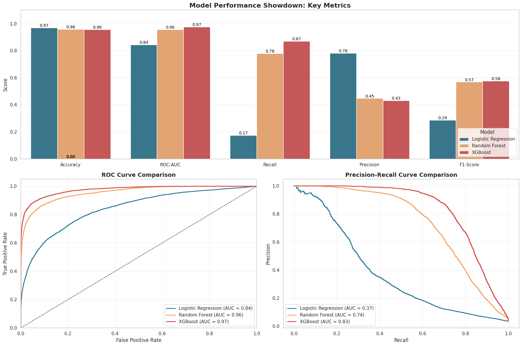
Final Verdict: XGBoost - The Undisputed Victor

Why XGBoost wins:

Highest Recall (Most Important for Fraud Detection)
- Logistic Regression: Recall 0.17 → misses most fraud.
- XGBoost: Recall 0.87 → detects the majority of fraudulent transactions.
Best Precision–Recall Performance
- XGBoost PR AUC: 0.83
- Logistic Regression PR AUC: 0.36 XGBoost handles class imbalance far more effectively.
Acceptable Precision Trade-off
- Logistic Regression Precision: 0.75
- XGBoost Precision: 0.43 Lower precision is acceptable since false negatives (missed fraud) are costlier than false positives.
Overall Strength
- ROC-AUC: 0.97 (highest among all models)

→ Final Choice: XGBoost It provides the strongest fraud detection performance and minimizes missed fraudulent activity.

EVALUATING ON UNSEEN DATA

The Final Trial: Judging on Unseen Cases

To ensure the integrity of our investigation, we cannot rely solely on the evidence we have already analyzed. We must sequester 5% of the transaction data into a digital “vault,” effectively creating a set of “cold cases” that our algorithms have never seen. By testing our final suspect profile against this untouched evidence, we prove that our model hasn’t just memorized the details of past crimes, but has genuinely learned to detect the fingerprints of fraud in the real world.

print("Final Check: Predictions on the Holdout Set...")

# 1. Make Predictions
y_pred_holdout = xgb_model.predict(X_holdout)

# 2. Retrieve TransactionIDs
holdout_ids = df_cleaned.loc[X_holdout.index, 'TransactionID']

# 3. Create a Results DataFrame
results_df = pd.DataFrame({
    'TransactionID': holdout_ids.values,
    'y_predicted': y_pred_holdout,
    'y_actual': y_holdout.values
})

# 4. Select 10 Fraud and 10 Non-Fraud Samples
sample_fraud = results_df[results_df['y_actual'] == 1].head(15)
sample_legit = results_df[results_df['y_actual'] == 0].head(15)

# 5. Combine into one table
final_display = pd.concat([sample_fraud, sample_legit])

holdout_accuracy = accuracy_score(y_holdout, y_pred_holdout)
holdout_auc = roc_auc_score(y_holdout, xgb_model.predict_proba(X_holdout)[:, 1])

print(f"Total Rows in Holdout: {len(y_holdout)}")
print(f"Holdout Accuracy:      {holdout_accuracy:.4f}")
print(f"Holdout ROC-AUC:       {holdout_auc:.4f}\n")

print(f"\nDisplaying {len(final_display)} sample rows from Holdout Set:")
print(final_display.to_string(index=False))

Final Check: Predictions on the Holdout Set...
Total Rows in Holdout: 29527
Holdout Accuracy:      0.9535
Holdout ROC-AUC:       0.9743


Displaying 30 sample rows from Holdout Set:
 TransactionID  y_predicted  y_actual
     3265024.0            1       1.0
     3338787.0            0       1.0
     3228012.0            1       1.0
     3288978.0            1       1.0
     3378820.0            1       1.0
     3494141.0            1       1.0
     3510134.0            1       1.0
     3409700.0            1       1.0
     3042258.0            1       1.0
     3475711.0            1       1.0
     3399748.0            1       1.0
     3320659.0            1       1.0
     3307507.0            1       1.0
     3335475.0            1       1.0
     3151082.0            1       1.0
     3495345.0            0       0.0
     3059907.0            0       0.0
     3568138.0            0       0.0
     3306214.0            0       0.0
     3395254.0            0       0.0
     3447490.0            0       0.0
     2999686.0            0       0.0
     3246309.0            0       0.0
     3076325.0            0       0.0
     3200308.0            0       0.0
     3222756.0            1       0.0
     3121241.0            0       0.0
     3118889.0            0       0.0
     3088558.0            0       0.0
     3222495.0            0       0.0

The Closure

The Unveiling of the Vault: Upon unlocking our 5% holdout set, the evidence completely sequestered from our training process, our XGBoost model achieved a ROC-AUC of 0.9743. In forensic terms, this means our suspect profile is incredibly robust, maintaining elite performance even on “cold cases” it had never seen before.

Evidence Analysis:

High Reliability (97.4% AUC): The model demonstrates an exceptional ability to rank fraudulent transactions higher than legitimate ones. It didn’t just memorize the case files; it learned the underlying modus operandi of the fraudsters.
Real-World Precision: Looking at our sample of 30 transactions, we see a high correlation between our predicted verdict and the actual truth. While no detective is perfect (we see a few false negatives where y_predicted=0 but y_actual=1), the system is vastly superior to random guessing or simple rules.

Impact: Implementing this system would likely save millions in chargeback losses while ensuring that the vast majority of legitimate customers can buy their party supplies without interruption.

🎬 CLOSING SCENE: Sarah’s new ending

png

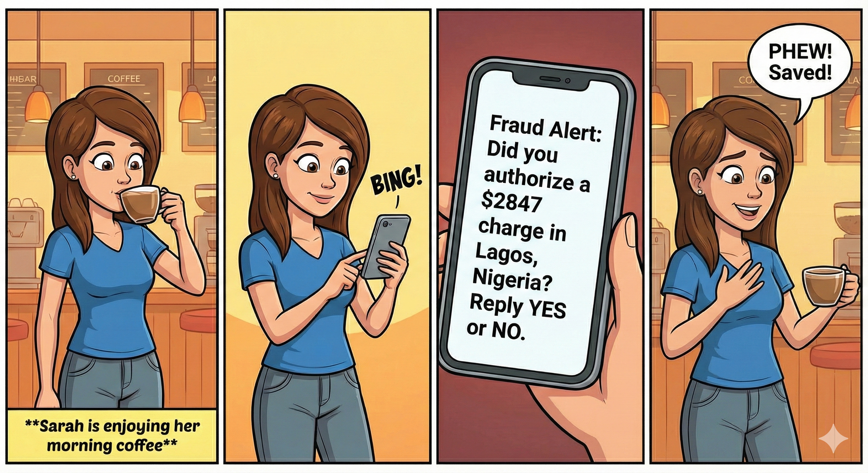
Future Work: The Next Frontier

As we look ahead, the next stage is to make our fraud detection system faster, clearer, and more adaptable. Moving from batch processing to real-time scoring will allow transactions to be evaluated within milliseconds, which is essential in real-world payment environments. Adding model explainability through tools like SHAP will help analysts and regulators understand exactly why a transaction was flagged. Because fraud patterns constantly change, we’ll also need automated retraining pipelines that detect when the model’s performance drops and update it accordingly. In the future, we can explore more advanced methods such as graph neural networks to capture relationships between users and transactions, and semi-supervised learning to take advantage of large volumes of unlabeled data. Together, these improvements will make the system more reliable and better equipped to adapt to evolving fraud behavior.

References & Resources

Data Source

IEEE-CIS Fraud Detection Dataset: Provided by Vesta Corporation.
Context: The dataset contains real-world e-commerce transactions with a wide range of features including device type, card details, and transaction time.

Methodologies & Libraries

Scikit-Learn: Used for data preprocessing (Scaling, Encoding), imputation, and baseline modeling (Logistic Regression, Random Forest).
XGBoost: Used for high-performance gradient boosting to detect complex fraud patterns.
Matplotlib & Seaborn: Used for visualizing the “Crime Scene” (EDA) and model performance (ROC Curves).

Further Reading

Fraud Detection using Machine Learning (IEEE Xplore)
Handling Imbalanced Datasets in Computer Vision and Fraud Detection